Numerical Partial Differential Equation IV: Spectral Methods

Weak Formulation

In mathematical modeling of physical systems, weak formulations provide a powerful framework to analyze and solve partial differential equations (PDEs). Unlike the traditional strong (or classical) formulations, which require the solution to be differentiable and satisfy the PDE everywhere in the domain, the weak formulation relaxes these requirements. Instead, it ensures that the PDE holds in an integral sense, allowing solutions that may be less regular.

Why Weak Formulations?

1. Broader Solution Space: Weak formulations permit solutions that are not differentiable everywhere, such as those with discontinuities or sharp gradients. This is particularly useful in real-world problems, such as fluid dynamics, where solutions often exhibit such features.

2. Natural Fit for Numerical Methods: Many numerical methods, including finite element and spectral methods, are based on weak formulations. These methods approximate the solution by projecting it onto a finite-dimensional space of basis functions, ensuring that the integral form of the equation is satisfied.

3. Conservation Laws: Weak formulations often align naturally with conservation laws, as they integrate the governing equations over a control volume or domain. This ensures that key physical quantities, such as mass, momentum, and energy, are preserved in the numerical approximation.

Key Idea of Weak Formulation

Given a PDE:

(583)\[\begin{align} \mathcal{L}(u) = f, \end{align}\]

where \(\mathcal{L}\) is a differential operator, \(u\) is the solution, and \(f\) is a source term, the weak formulation is derived by multiplying the equation by a test function \(v\) and integrating over the domain \(\Omega\):

(584)\[\begin{align} \int_\Omega v \, \mathcal{L}(u) \, d\Omega = \int_\Omega v \, f \, d\Omega. \end{align}\]

Through integration by parts, derivatives on \(u\) are shifted onto \(v\), reducing the regularity requirements on \(u\). For example, the weak form of the Poisson equation:

(585)\[\begin{align} -\nabla^2 u = f, \end{align}\]

becomes:

(586)\[\begin{align} \int_\Omega \nabla v \cdot \nabla u \, d\Omega = \int_\Omega v f \, d\Omega. \end{align}\]

Here, \(u\) needs only to be square-integrable, rather than twice differentiable, making the formulation more flexible.

Connection to Spectral Methods

Spectral methods build directly on the weak formulation by representing the solution \(u\) and test functions \(v\) as expansions in terms of orthogonal basis functions (e.g., Fourier modes or polynomials). The PDE is then projected onto these basis functions, leading to a system of algebraic equations for the coefficients of the expansion.

The transition from weak formulations to spectral methods highlights the elegance and power of this approach: by working in function spaces tailored to the problem, spectral methods achieve high accuracy and efficiency in solving PDEs, particularly for smooth solutions in periodic domains.

Introduction to Spectral Methods

Spectral methods are a powerful class of numerical techniques used to solve partial differential equations (PDEs) by representing the solution as a global expansion of orthogonal basis functions. Unlike finite difference or finite volume methods, which approximate the solution locally at discrete grid points, spectral methods leverage the smoothness of the solution to achieve high accuracy with fewer degrees of freedom. This makes spectral methods particularly suitable for problems involving smooth and periodic solutions, such as fluid dynamics and wave propagation.

Why Use Spectral Methods?

1. High Accuracy: Spectral methods are renowned for their ability to achieve exponential convergence rates for smooth solutions. By representing the solution as a sum of global basis functions, spectral methods resolve fine details with far fewer grid points compared to traditional numerical methods.

2. Efficient Computation: Operations such as differentiation and integration become algebraic manipulations in spectral space. This allows for fast and efficient computation, especially when coupled with Fast Fourier Transforms (FFT).

3. Energy-Conserving Properties: By carefully choosing the basis functions and truncating higher-order modes (Galerkin truncation), spectral methods naturally conserve key physical quantities like energy and enstrophy. This property is critical in applications such as turbulence modeling and geophysical fluid dynamics.

4. Applications in Science and Engineering: Spectral methods are widely used in areas such as:

   • Astrophysical fluid dynamics.

   • Weather prediction and ocean modeling.

   • Quantum mechanics and wave phenomena.

Core Idea of Spectral Methods

The central idea of spectral methods is to approximate a function \(u(x)\) as a series of orthogonal basis functions. For example, in the Fourier spectral method, the function is expanded as:

(587)\[\begin{align} u(x) = \sum_{k=-N/2}^{N/2} \hat{u}_k e^{i k x}, \end{align}\]

where \(\hat{u}_k\) are the Fourier coefficients representing the contribution of each basis function. The advantage of this representation is that operations like differentiation transform into simple multiplications in spectral space. For example:

(588)\[\begin{align} \frac{\partial u}{\partial x} = \sum_{k=-N/2}^{N/2} i k \hat{u}_k e^{i k x}. \end{align}\]

This property drastically simplifies the computation of derivatives, making spectral methods particularly attractive for solving PDEs.

import numpy as np
from numpy.fft  import fft2, ifft2
from matplotlib import pyplot as plt
from tqdm import tqdm

Lx = 2 * np.pi # Domain size
Nx = 128       # Number of grid points

x  = np.linspace(-Lx/2, Lx/2, Nx, endpoint=False)
kx = np.fft.fftfreq(Nx, d=Lx/Nx) * 2 * np.pi

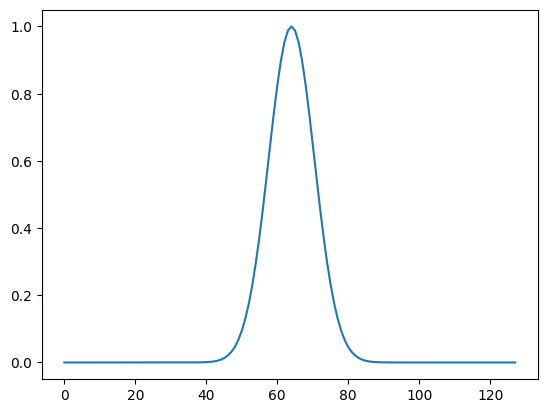
f = np.exp(-0.5 * (x*x) / 0.1)
plt.plot(f)

[<matplotlib.lines.Line2D at 0x7fa34828de80>]

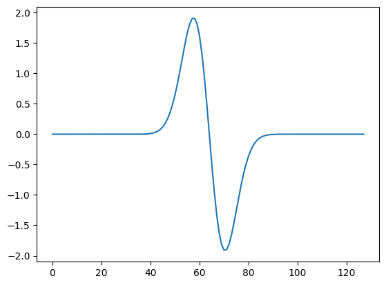
g_exact = -x * np.exp(-0.5 * (x*x) / 0.1) / 0.1
plt.plot(g_exact)

[<matplotlib.lines.Line2D at 0x7fa3482d1dc0>]

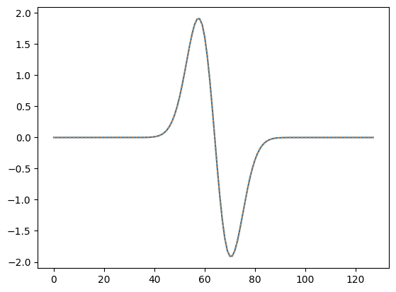
F = np.fft.fft(f)
G = 1j * kx * F
g = np.fft.ifft(G).real

plt.plot(g_exact)
plt.plot(g, ':')

np.max(abs(g - g_exact))

np.float64(1.709743457922741e-14)

Periodic vs. Non-Periodic Domains

Spectral methods are naturally suited to periodic domains, where Fourier basis functions \(e^{i k x}\) form an orthogonal basis. For non-periodic problems, alternative basis functions like Chebyshev polynomials or Legendre polynomials are used. These basis functions maintain the accuracy of spectral methods while adapting to non-periodic boundary conditions.

Strengths

• Exponential Convergence: For smooth problems, spectral methods outperform traditional numerical methods in terms of accuracy.

• Global Representation: Captures global features of the solution with fewer degrees of freedom.

• Efficiency with FFT: Fast Fourier Transforms enable rapid computation of spectral coefficients.

Limitations

• Smoothness Requirement: Spectral methods perform poorly for non-smooth or discontinuous solutions, where the Gibbs phenomenon introduces oscillations.

• Complexity for Non-Periodic Domains: Implementing spectral methods for non-periodic problems requires specialized basis functions and quadrature rules.

• Global Coupling: Each mode influences the entire domain, which can lead to computational challenges for very large systems.

Spectral Methods in Fluid Dynamics

In fluid dynamics, spectral methods are commonly used to solve the incompressible Navier-Stokes equations. By transforming the equations into spectral space, the nonlinear terms can be computed efficiently while maintaining conservation properties. For incompressible flows, the vorticity-streamfunction formulation is particularly suitable, as it eliminates the pressure term and reduces the computational complexity.

In this lecture, we will focus on applying spectral methods to solve the 2D incompressible hydrodynamics equations. Specifically, we will:

1. Derive the governing equations in spectral space.

2. Discuss the vorticity-streamfunction formulation and its advantages.

3. Implement a spectral solver to simulate the evolution of vorticity in a 2D periodic domain.

This introduction sets the stage for understanding how spectral methods leverage mathematical elegance and computational efficiency to solve complex PDEs with remarkable accuracy.

Introduction to 2D Incompressible Hydrodynamics

The hydrodynamic equations govern the conservation of mass and momentum in a fluid. In their compressible form (that we derived in previous lectures), they are written as:

(589)\[\begin{align} \frac{\partial \rho}{\partial t} + \nabla \cdot (\rho \mathbf{u}) &= 0, \quad \text{(Continuity Equation)} \\ \frac{\partial (\rho \mathbf{u})}{\partial t} + \nabla \cdot (\rho \mathbf{u} \mathbf{u}) &= -\nabla p + \mu \nabla^2 \mathbf{u} + \mathbf{f}, \quad \text{(Momentum Equation)} \end{align}\]

where:

• \(\rho\) is the density,

• \(\mathbf{u}\) is the velocity field,

• \(p\) is the pressure,

• \(\mu\) is the dynamic viscosity,

• \(\mathbf{f}\) is an external force.

In the incompressible limit, the sound speed approaches infinite \(c \rightarrow \infty\). For simplicity, the density \(\rho\) can be assumed constant, and the continuity equation reduces to the incompressibility condition:

(590)\[\begin{align} \nabla \cdot \mathbf{u} = 0. \end{align}\]

Substituting this condition into the momentum equation simplifies the Navier-Stokes equations to:

(591)\[\begin{align} \frac{\partial \mathbf{u}}{\partial t} + (\mathbf{u} \cdot \nabla) \mathbf{u} = -\nabla p + \nu \nabla^2 \mathbf{u} + \mathbf{f}, \end{align}\]

where \(\nu = \mu / \rho\) is the kinematic viscosity. These equations describe the flow of incompressible fluids and are widely used in modeling small-scale laboratory experiments and large-scale geophysical flows.

While the incompressible Navier-Stokes equations also apply to three-dimensional flows, many physical systems can be effectively approximated as two-dimensional. For example:

• Atmospheric flows and ocean currents are largely horizontal due to their vast spatial extent compared to their depth.

• Thin liquid films and confined flows are geometrically restricted to two dimensions.

In 2D, the dynamics exhibit unique features that distinguish them from 3D flows:

Conservation of Enstrophy

In 2D, the vorticity \(w = \nabla \times \mathbf{u}\) is a scalar field. Its evolution is governed by the vorticity transport equation, which conserves both energy and enstrophy in the absence of dissipation:

(592)\[\begin{align} E &= \frac{1}{2} \int |\mathbf{u}|^2 \, dx \, dy\\ Z &= \frac{1}{2} \int w^2 \, dx \, dy. \end{align}\]

Energy conservation governs the total kinetic energy of the system, while enstrophy conservation introduces a second constraint that strongly influences the flow dynamics.

Inverse Energy Cascade

A striking feature of 2D turbulence is the inverse energy cascade. In 3D turbulence, energy flows from large scales (low wavenumbers) to small scales (high wavenumbers) and is dissipated by viscosity. In 2D, however, energy flows in the opposite direction, from small scales to large scales, leading to the formation of large, coherent structures like cyclones and anticyclones. This behavior is directly tied to the dual conservation of energy and enstrophy.

Vorticity-Streamfunction Formulation

To simplify the mathematical and computational treatment of 2D incompressible hydrodynamics, the governing equations are often reformulated in terms of the vorticity \(w\) and the streamfunction \(\psi\). This formulation has several advantages: it eliminates the pressure term from the equations, reduces the number of variables, and ensures incompressibility is automatically satisfied. In this section, we derive the vorticity-streamfunction formulation, define the Jacobian determinant to handle the nonlinear advection term, and introduce additional physical effects such as Ekman damping and the beta-plane approximation.

Definitions and Key Relationships

For 2D incompressible flows, the velocity field \(\mathbf{u} = (u_x, u_y)\) can be expressed in terms of a scalar function, the streamfunction \(\psi(x, y, t)\), as:

(593)\[\begin{align} \mathbf{u} = \nabla \times (\psi \mathbf{\hat{z}}), \end{align}\]

where \(\mathbf{\hat{z}}\) is the unit vector perpendicular to the 2D plane. In component form:

(594)\[\begin{align} u_x = \frac{\partial \psi}{\partial y}, \quad u_y = -\frac{\partial \psi}{\partial x}. \end{align}\]

This representation automatically satisfies the incompressibility condition:

(595)\[\begin{align} \nabla \cdot \mathbf{u} = \frac{\partial u_x}{\partial x} + \frac{\partial u_y}{\partial y} = 0. \end{align}\]

The vorticity \(w\) is a scalar quantity in 2D, defined as the curl of the velocity field:

(596)\[\begin{align} w = \nabla \times \mathbf{u}. \end{align}\]

Using the velocity components in terms of the streamfunction, the vorticity can be written as:

(597)\[\begin{align} w = \frac{\partial u_y}{\partial x} - \frac{\partial u_x}{\partial y} = -\nabla^2 \psi. \end{align}\]

Thus, the vorticity and streamfunction are related by the Poisson equation:

(598)\[\begin{align} w = -\nabla^2 \psi. \end{align}\]

This relationship allows the velocity field to be computed from the vorticity by solving the Poisson equation for \(\psi\), and then taking derivatives of \(\psi\) to find \(u_x\) and \(u_y\).

Governing Equation for Vorticity

The vorticity transport equation is derived from the incompressible Navier-Stokes equations. Taking the curl of the momentum equation eliminates the pressure gradient term, yielding:

(599)\[\begin{align} \frac{\partial w}{\partial t} + \mathbf{u} \cdot \nabla w = \nu \nabla^2 w + \mathbf{f}_w, \end{align}\]

where:

• \(\mathbf{u} \cdot \nabla w\) represents the nonlinear advection of vorticity,

• \(\nu \nabla^2 w\) accounts for viscous diffusion,

• \(\mathbf{f}_w\) is the vorticity-specific forcing term.

The term \(\mathbf{u} \cdot \nabla w\) can be expanded using the velocity components as:

(600)\[\begin{align} \mathbf{u} \cdot \nabla w = u_x \frac{\partial w}{\partial x} + u_y \frac{\partial w}{\partial y}. \end{align}\]

By substituting \(u_x\) and \(u_y\) in terms of \(\psi\), the nonlinear advection term is rewritten as the Jacobian determinant:

(601)\[\begin{align} J(\psi, w) = \frac{\partial \psi}{\partial x} \frac{\partial w}{\partial y} - \frac{\partial \psi}{\partial y} \frac{\partial w}{\partial x}. \end{align}\]

Thus, the vorticity transport equation becomes:

(602)\[\begin{align} \frac{\partial w}{\partial t} - J(\psi, w) = \nu \nabla^2 w + \mathbf{f}_w. \end{align}\]

Incorporating Additional Physical Effects

Ekman damping models frictional effects caused by the interaction of the fluid with a boundary layer. It acts as a large-scale energy sink and is proportional to the vorticity:

(603)\[\begin{align} -\mu w, \end{align}\]

where \(\mu\) is the Ekman coefficient. Including this term in the vorticity transport equation gives:

(604)\[\begin{align} \frac{\partial w}{\partial t} - J(\psi, w) = \nu \nabla^2 w - \mu w + \mathbf{f}_w. \end{align}\]

Ekman damping is particularly relevant in geophysical systems, where it represents energy dissipation due to the Earth’s surface or ocean floors.

The \(\beta\)-plane approximation models the variation of the Coriolis parameter \(f\) with latitude. In the vorticity equation, this introduces a term proportional to the northward velocity component \(u_y\):

(605)\[\begin{align} \beta u_y, \end{align}\]

where \(\beta\) is the linear expansion coefficient of the Coriolis parameter. Including this term in the vorticity transport equation gives:

(606)\[\begin{align} \frac{\partial w}{\partial t} - J(\psi, w) + \beta u_y = \nu \nabla^2 w - \mu w + \mathbf{f}_w. \end{align}\]

The beta-plane term is crucial for studying large-scale atmospheric and oceanic dynamics, as it leads to phenomena such as Rossby waves and geostrophic turbulence.

Advantages of the Vorticity-Streamfunction Formulation

1. Elimination of Pressure: The pressure term, which requires solving an additional Poisson equation in the velocity-pressure formulation, is completely removed in the vorticity-streamfunction approach.

2. Reduced Number of Variables: By working with \(w\) and \(\psi\), the system is reduced to a single scalar equation for \(w\) coupled with the Poisson equation for \(\psi\).

3. Natural Compatibility with Spectral Methods: The vorticity-streamfunction formulation lends itself well to spectral methods. Derivatives of \(w\) and \(\psi\) are straightforward to compute in spectral space, and the Poisson equation becomes an algebraic equation.

4. Incorporation of Geophysical Effects: Ekman damping and the beta-plane approximation extend the applicability of the formulation to real-world problems in atmospheric and oceanic sciences.

Spectral Representation of the Equations

The vorticity-streamfunction formulation simplifies the governing equations of 2D incompressible hydrodynamics, making them naturally suited to spectral methods. By representing the vorticity and streamfunction in terms of Fourier series, we can efficiently compute derivatives and nonlinear terms in spectral space. This section details the spectral representation of the vorticity transport equation and the Poisson equation, highlighting the mathematical transformations, strategies to handle aliasing errors, and implementation in Python.

Fourier Representation of Vorticity and Streamfunction

For a periodic domain of size \(L_x \times L_y\), the vorticity \(w(x, y, t)\) and streamfunction \(\psi(x, y, t)\) can be expanded as Fourier series:

(607)\[\begin{align} w(x, y, t) &= \sum_{k_x, k_y} \hat{w }_{k_x, k_y}(t) e^{i (k_x x + k_y y)}, \\ \psi(x, y, t) &= \sum_{k_x, k_y} \hat{\psi}_{k_x, k_y}(t) e^{i (k_x x + k_y y)}, \end{align}\]

where:

• \(\hat{w}_{k_x, k_y}\) and \(\hat{\psi}_{k_x, k_y}\) are the Fourier coefficients of vorticity and streamfunction, respectively.

• \(k_x\) and \(k_y\) are the wavenumbers in the \(x\)- and \(y\)-directions, given by:

  (608)\[\begin{align} k_x = \frac{2\pi n_x}{L_x}, \quad k_y = \frac{2\pi n_y}{L_y}, \quad n_x, n_y \in \mathbb{Z}. \end{align}\]

Fourier Differentiation

In spectral space, derivatives with respect to \(x\) and \(y\) transform into simple multiplications by \(ik_x\) and \(ik_y\), respectively. For example:

(609)\[\begin{align} \frac{\partial w}{\partial x} \rightarrow ik_x \hat{w}_{k_x, k_y}, \quad \frac{\partial^2 w}{\partial x^2} \rightarrow -k_x^2 \hat{w}_{k_x, k_y}. \end{align}\]

This property makes spectral methods computationally efficient, as derivatives reduce to element-wise multiplications.

Poisson Equation in Spectral Space

The Poisson equation relates the vorticity \(w\) and the streamfunction \(\psi\):

(610)\[\begin{align} w = -\nabla^2 \psi. \end{align}\]

In Fourier space, the Laplacian \(\nabla^2\) becomes multiplication by \(-k^2\), where \(k^2 = k_x^2 + k_y^2\). Thus, the Poisson equation transforms into:

(611)\[\begin{align} \hat{\psi}_{k_x, k_y} = \frac{\hat{w}_{k_x, k_y}}{k^2}, \quad k^2 \neq 0. \end{align}\]

The \(k^2 = 0\) mode corresponds to the mean value of \(\psi\), which can be set to zero for flows with no net circulation.

(612)\[\begin{align} u_y = -\frac{\partial \psi}{\partial x}. \end{align}\]

Vorticity Transport Equation in Spectral Space

Recalling the vorticity transport equation in real space is:

(613)\[\begin{align} \frac{\partial w}{\partial t} - J(\psi, w) + \beta u_y = \nu \nabla^2 w - \mu w + \mathbf{f}_w. \end{align}\]

In spectral space:

• The Laplacian term \(\nabla^2 w\) transforms into \(-k^2 \hat{w}_{k_x, k_y}\).

• The Ekman damping term \(\mu w\) becomes \(-\mu \hat{w}_{k_x, k_y}\).

• The Coriolis term \(\beta u_y\) becomes \(-\beta ik_x \hat{w}_{k_x, k_y}/k^2\).

• The nonlinear term \(J(\psi, w)\) is evaluated in real space and transformed back to spectral space using the Fast Fourier Transform (FFT).

The equation in spectral space becomes:

(614)\[\begin{align} \frac{\partial}{\partial t}\hat{w}_{k_x, k_y} = \widehat{J(\psi, w)} - \nu k^2 \hat{w}_{k_x, k_y} - \mu \hat{w}_{k_x, k_y} + \beta \frac{ik_x \hat{w}_{k_x, k_y}}{k^2} + \hat{f}_{w k_x, k_y}. \end{align}\]

# Define the grid and wavenumbers
Lx, Ly = 2 * np.pi, 2 * np.pi  # Domain size
Nx, Ny = 128, 128              # Number of grid points

x = np.linspace(-Lx/2, Lx/2, Nx, endpoint=False)
y = np.linspace(-Lx/2, Ly/2, Ny, endpoint=False)
x, y = np.meshgrid(x, y)

kx = np.fft.fftfreq(Nx, d=Lx/Nx) * 2 * np.pi
ky = np.fft.fftfreq(Ny, d=Ly/Ny) * 2 * np.pi
kx, ky = np.meshgrid(kx, ky)

kk  = kx*kx + ky*ky
ikk = 1.0 / (kk + 1.2e-38)
ikk[0,0] = 0  # Avoid multiplied by infinity for mean mode

# Initialize vorticity and streamfunction in spectral space
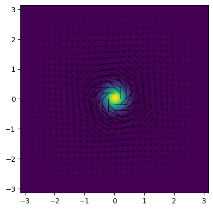
w = np.exp(-0.5*(x*x+y*y)*16) # Example initial vorticity

# Transform to Fourier (spectral) space
W   = fft2(w)
Psi = ikk * W

# Obtain velocity field
def vel(psi):
    psi_x = ifft2(1j * kx * fft2(psi)).real
    psi_y = ifft2(1j * ky * fft2(psi)).real
    return psi_y, -psi_x

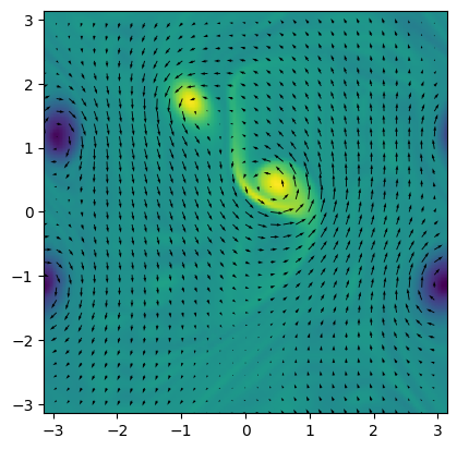
def plot(W, skip=4):
    psi    = ifft2(ikk * W).real
    ux, uy = vel(psi)
    plt.imshow(ifft2(W).real, origin='lower', extent=[-Lx/2,Lx/2,-Ly/2,Ly/2])
    plt.quiver(x[::skip,::skip], y[::skip,::skip], ux[::skip,::skip], uy[::skip,::skip])

plot(W)

# Compute Jacobian determinant in real space
def Jdet(Psi, W):
    psi_x = ifft2(1j * kx * Psi).real
    psi_y = ifft2(1j * ky * Psi).real
    w_x   = ifft2(1j * kx * W  ).real
    w_y   = ifft2(1j * ky * W  ).real
    return fft2(psi_x * w_y - psi_y * w_x)

J = Jdet(Psi, W)
print(np.max(ifft2(J).imag))

2.7371971311652333e-21

Handling Aliasing Errors

Nonlinear terms, such as \(J(\psi, w)\), involve products in real space that translate into convolutions in spectral space. These convolutions can introduce spurious interactions between modes, known as aliasing errors, due to the finite resolution of the grid.

The 2/3 rule is a widely used de-aliasing technique that truncates Fourier modes beyond \(2/3\) of the maximum wavenumber. For a grid with \(N\) points in each dimension:

• Retain modes for \(|k_x|, |k_y| \leq N/3\).

• Set all other modes to zero.

The 2/3 rule ensures that spurious contributions from nonlinear interactions fall outside the resolved spectral range.

# Apply the 2/3 rule
def dealiasing(F):
    Hx = Nx // 3
    Hy = Ny // 3
    F[Hx:-Hx+1, :] = 0
    F[:, Hy:-Hy+1] = 0
    return F

# Apply de-aliasing to the Jacobian
J = dealiasing(J)
print(np.max(ifft2(J).imag))

2.618213643193911e-21

Spectral-Galerkin vs. Pseudo-Spectral Methods

The spectral-Galerkin method projects the governing equations onto the basis functions of the spectral expansion. This ensures the residual is orthogonal to the retained modes.

The pseudo-spectral method evaluates nonlinear terms in real space and transforms them back to spectral space using FFT. While computationally efficient, it often requires de-aliasing or explicit viscosity to control aliasing errors. This method balances speed and accuracy, making it popular for practical simulations.

Time Integration of the Spectral Equations

After reformulating the vorticity-streamfunction equations in spectral space, the next step is to integrate the vorticity transport equation in time. Time integration involves advancing the Fourier coefficients of vorticity \(\hat{w}_{k_x, k_y}\) while accurately handling the nonlinear and linear terms. This section discusses suitable time-stepping schemes, their implementation, and how they are applied to the spectral representation of the equations.

Time-Stepping Schemes

Time integration methods for the spectral vorticity transport equation must balance stability, accuracy, and computational efficiency. Two commonly used schemes in spectral methods are:

Explicit Schemes

Explicit schemes, such as the Runge-Kutta (RK) family, compute the solution at the next time step based on known quantities at the current time step. They are easy to implement and efficient for problems dominated by advection or nonlinear dynamics.

Implicit Schemes

Implicit schemes, such as Crank-Nicolson, are unconditionally stable for linear terms but require solving a system of equations at each time step.

Semi-Implicit Methods

In spectral methods, implicit schemes are often used for the linear terms (e.g., viscous diffusion) to allow larger time steps, while explicit schemes handle nonlinear terms.

A common approach splits the equation into linear and nonlinear parts:

(615)\[\begin{align} \frac{\partial \hat{w}}{\partial t} = L(\hat{w}) + N(\hat{w}), \end{align}\]

where:

• \(L(\hat{w})\) represents linear terms (e.g., viscous diffusion, Ekman damping, Coriolis effects),

• \(N(\hat{w})\) represents nonlinear terms (e.g., Jacobian).

The linear terms are treated implicitly, while the nonlinear terms are advanced explicitly. For example, the time-discretized form is:

(616)\[\begin{align} \hat{w}^{n+1} = \frac{\hat{w}^n + \Delta t N(\hat{w}^n)}{1 - \Delta t L}. \end{align}\]

This approach combines the stability of implicit methods with the simplicity of explicit methods.

Time Integration of the Vorticity Transport Equation

The spectral vorticity transport equation is:

(617)\[\begin{align} \frac{\partial}{\partial t}\hat{w}_{k_x, k_y} = \widehat{J(\psi, w)} - \nu k^2 \hat{w}_{k_x, k_y} - \mu \hat{w}_{k_x, k_y} + \beta \frac{ik_x \hat{w}_{k_x, k_y}}{k^2} + \hat{f}_{w k_x, k_y}. \end{align}\]

Breaking this into linear and nonlinear parts:

• Linear Terms: Viscous diffusion \(-\nu k^2 \hat{w}\), Ekman damping \(-\mu \hat{w}\), and Coriolis effect \(\beta ik_x \hat{w}/k^2\).

• Nonlinear Terms: Jacobian determinant \(\widehat{J(\psi, w)}\).

Using a semi-implicit scheme:

1. Advance the nonlinear terms explicitly using an RK4 method.

2. Solve the linear terms implicitly using the formula:

   (618)\[\begin{align} \hat{w}_{k_x, k_y}^{n+1} = \frac{\hat{w}_{k_x, k_y}^n + \Delta t N(\hat{w}_{k_x, k_y}^n)}{1 + \Delta t (\nu k^2 + \mu - \beta ik_x/k^2)}. \end{align}\]

# Initialize vorticity and streamfunction in spectral space
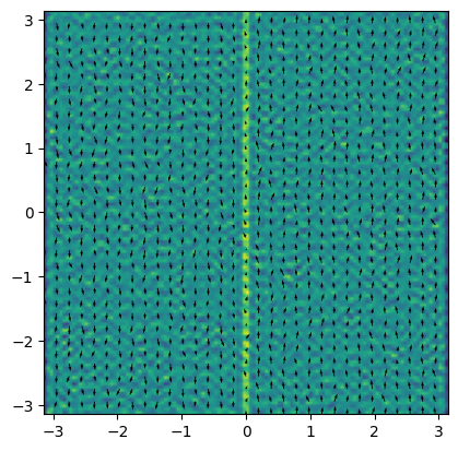
ux = np.random.normal(scale=0.5, size=x.shape)
uy = np.where(x >= 0, 1, -1) # Example initial vorticity

W = dealiasing(1j * kx * fft2(uy) - 1j * ky * fft2(ux))
plot(W)

# Define simulation parameters
dt   = 0.001  # Time step
nu   = 0.001  # Viscosity
mu   = 0.0    # Ekman damping
beta = 0.0    # Coriolis parameter
N    = 10000  # Number of time steps
S    = 250

# Time-stepping loop
for n in tqdm(range(N//S)):
    plot(W)
    plt.savefig(f'{n:04d}.png', dpi=300, bbox_inches='tight')
    plt.close()

    for j in range(S):
        # Obtain stream function
        Psi = ikk * W

        # Compute nonlinear term (Jacobian determinant)
        J = Jdet(Psi, W)
        J = dealiasing(J)  # Apply 2/3 rule

        # Update vorticity in spectral space
        W = (W + dt * J) / (1 + dt * (nu * kk + mu - (1j * beta) * (kx * ikk)))

plot(W)
plt.savefig(f'{n+1:04d}.png', dpi=300, bbox_inches='tight')

  0%|          | 0/40 [00:00<?, ?it/s]

  2%|▎         | 1/40 [00:00<00:22,  1.72it/s]

  5%|▌         | 2/40 [00:01<00:21,  1.73it/s]

  8%|▊         | 3/40 [00:01<00:21,  1.75it/s]

 10%|█         | 4/40 [00:02<00:20,  1.74it/s]

 12%|█▎        | 5/40 [00:02<00:20,  1.74it/s]

 15%|█▌        | 6/40 [00:03<00:19,  1.74it/s]

 18%|█▊        | 7/40 [00:04<00:19,  1.69it/s]

 20%|██        | 8/40 [00:04<00:18,  1.71it/s]

 22%|██▎       | 9/40 [00:05<00:18,  1.72it/s]

 25%|██▌       | 10/40 [00:05<00:17,  1.72it/s]

 28%|██▊       | 11/40 [00:06<00:16,  1.71it/s]

 30%|███       | 12/40 [00:06<00:16,  1.72it/s]

 32%|███▎      | 13/40 [00:07<00:15,  1.72it/s]

 35%|███▌      | 14/40 [00:08<00:15,  1.73it/s]

 38%|███▊      | 15/40 [00:08<00:14,  1.73it/s]

 40%|████      | 16/40 [00:09<00:13,  1.74it/s]

 42%|████▎     | 17/40 [00:09<00:13,  1.74it/s]

 45%|████▌     | 18/40 [00:10<00:12,  1.74it/s]

 48%|████▊     | 19/40 [00:10<00:12,  1.74it/s]

 50%|█████     | 20/40 [00:11<00:11,  1.69it/s]

 52%|█████▎    | 21/40 [00:12<00:11,  1.71it/s]

 55%|█████▌    | 22/40 [00:12<00:10,  1.72it/s]

 57%|█████▊    | 23/40 [00:13<00:09,  1.72it/s]

 60%|██████    | 24/40 [00:13<00:09,  1.72it/s]

 62%|██████▎   | 25/40 [00:14<00:08,  1.73it/s]

 65%|██████▌   | 26/40 [00:15<00:08,  1.72it/s]

 68%|██████▊   | 27/40 [00:15<00:07,  1.73it/s]

 70%|███████   | 28/40 [00:16<00:06,  1.73it/s]

 72%|███████▎  | 29/40 [00:16<00:06,  1.74it/s]

 75%|███████▌  | 30/40 [00:17<00:05,  1.74it/s]

 78%|███████▊  | 31/40 [00:17<00:05,  1.75it/s]

 80%|████████  | 32/40 [00:18<00:04,  1.75it/s]

 82%|████████▎ | 33/40 [00:19<00:04,  1.75it/s]

 85%|████████▌ | 34/40 [00:19<00:03,  1.68it/s]

 88%|████████▊ | 35/40 [00:20<00:02,  1.70it/s]

 90%|█████████ | 36/40 [00:20<00:02,  1.71it/s]

 92%|█████████▎| 37/40 [00:21<00:01,  1.73it/s]

 95%|█████████▌| 38/40 [00:22<00:01,  1.73it/s]

 98%|█████████▊| 39/40 [00:22<00:00,  1.73it/s]

100%|██████████| 40/40 [00:23<00:00,  1.73it/s]

100%|██████████| 40/40 [00:23<00:00,  1.73it/s]