ODE Lab III: Advanced Topics#
The Double Pendulum Problem#
The double pendulum is a well known example of a non-linear, chaotic system in classical mechanics. It consists of a pendulum with another pendulum attached to its end, resulting in a system with two degrees of freedom. This configuration leads to highly complex and sensitive-dependent dynamics, making the double pendulum an excellent subject for studying chaos theory and non-linear dynamics. Because it is not possible to construct analytical solutions, it is also a great example to numerical integrators.

The equation of motion for double pendulum is pretty ugly. To set up the equations, we assume:
The two arms of the pendulums have the same length \(l\).
The mass of each arm is \(m\).
The angle between the first and second pendulums, with respect to the vertical axis, are denoted by \(\theta_1\) and \(\theta_2\).
Newton’s second law suggests that we will need to solve a system of two second-order ordinary differential equations (ODEs). Using the methods we learn in the lecture, we can cast the problem into a system of four first-order ODEs.
where \(p_1\) and \(p_2\) are called the generalized momenta. (There might be typos in the equation. Please double check.)
It would be impossible to implement this in a few minutes as a hands-on exercise!
Thankfully, we have just learned computational Lagrangian mechanics in class using autodiff and ODE integrator. The Lagrangian of the double pendulum system is:
We will use this to implement a solver in this hands-on lab.
! pip install jax
Requirement already satisfied: jax in /opt/hostedtoolcache/Python/3.12.10/x64/lib/python3.12/site-packages (0.6.0)
Requirement already satisfied: jaxlib<=0.6.0,>=0.6.0 in /opt/hostedtoolcache/Python/3.12.10/x64/lib/python3.12/site-packages (from jax) (0.6.0)
Requirement already satisfied: ml_dtypes>=0.5.0 in /opt/hostedtoolcache/Python/3.12.10/x64/lib/python3.12/site-packages (from jax) (0.5.1)
Requirement already satisfied: numpy>=1.25 in /opt/hostedtoolcache/Python/3.12.10/x64/lib/python3.12/site-packages (from jax) (2.2.5)
Requirement already satisfied: opt_einsum in /opt/hostedtoolcache/Python/3.12.10/x64/lib/python3.12/site-packages (from jax) (3.4.0)
Requirement already satisfied: scipy>=1.11.1 in /opt/hostedtoolcache/Python/3.12.10/x64/lib/python3.12/site-packages (from jax) (1.15.2)
import jax
jax.config.update("jax_enable_x64", True)
from jax import numpy as np
# Step 1. Copy an ODE Integrator from the class note

a =[
    [],
    [1/5],
    [3/40, 9/40],
    [44/45, -56/15, 32/9],
    [19372/6561, -25360/2187, 64448/6561, -212/729],
    [9017/3168, -355/33, 46732/5247, 49/176, -5103/18656],
    [35/384, 0, 500/1113, 125/192, -2187/6784, 11/84],
]

b_high = [35/384, 0, 500/1113, 125/192, -2187/6784, 11/84, 0] # Fifth-order accurate solution estimate
b_low  = [5179/57600, 0, 7571/16695, 393/640, -92097/339200, 187/2100, 1/40] # Fourth-order accurate solution estimate

c = [0, 1/5, 3/10, 4/5, 8/9, 1, 1]

def DP45_step(f, x, t, dt):
        # Compute intermediate k1 to k7
    k1 = f(x)
    k2 = f(x + dt*(a[1][0]*k1))
    k3 = f(x + dt*(a[2][0]*k1 + a[2][1]*k2))
    k4 = f(x + dt*(a[3][0]*k1 + a[3][1]*k2 + a[3][2]*k3))
    k5 = f(x + dt*(a[4][0]*k1 + a[4][1]*k2 + a[4][2]*k3 + a[4][3]*k4))
    k6 = f(x + dt*(a[5][0]*k1 + a[5][1]*k2 + a[5][2]*k3 + a[5][3]*k4 + a[5][4]*k5))
    k7 = f(x + dt*(a[6][0]*k1 + a[6][1]*k2 + a[6][2]*k3 + a[6][3]*k4 + a[6][4]*k5 + a[6][5]*k6))

    ks = [k1, k2, k3, k4, k5, k6, k7]

    # Compute high and low order estimates
    x_high = x
    for b, k in zip(b_high, ks):
        x_high += dt * b * k

    x_low  = x
    for b, k in zip(b_low, ks):
        x_low += dt * b * k

    return x_high, x_low, ks

def dt_update(dt, error, tol, fac=0.9, fac_min=0.1, fac_max=4.0, alpha=0.2):
    if error == 0:
        s = fac_max
    else:
        s = fac * (tol / error) ** alpha
    s = min(fac_max, max(fac_min, s))
    dt_new = dt * s
    return dt_new

def odeint(f, x, t, T, dt=0.1, atol=1e-6, rtol=1e-6):

    Ts = [t]
    Xs = [np.array(x)]

    while t < T:
        if t + dt > T:
            dt = T - t  # Adjust step size to end exactly at tf

        # Perform a single Dormand–Prince step
        x_high, x_low, _ = DP45_step(f, x, t, dt)

        # Compute the error estimate
        error = np.linalg.norm(x_high - x_low, ord=np.inf)

        # Compute the tolerance
        tol = atol + rtol * np.linalg.norm(x_high, ord=np.inf)

        # Check if the step is acceptable
        if error <= tol:
            # Accept the step
            t += dt
            x = x_high
            Ts.append(t)
            Xs.append(x)

        # Compute the new step size
        dt = dt_update(dt, error, tol)

    return np.array(Ts), np.array(Xs)
# Step 2. Copy ELrhs() from the class note

from jax import grad, jacfwd, jit
from jax.numpy.linalg import inv

def ELrhs(L):

    Lx  = grad(L, argnums=0)
    Lv  = grad(L, argnums=1)
    Lvp = jacfwd(Lv, argnums=(0,1))

    @jit
    def rhs(xv):
        x,   v   = xv
        Lvx, Lvv = Lvp(x, v)
        a = inv(Lvv) @ (Lx(x, v) - v @ Lvx)
        return np.array([v, a])

    return rhs
# Step 3. Combine ELrhs() with the ODE Integrator.  See, e.g., path() from class

def path(L, xv0, t0, t1, dt=0.1, atol=1e-6, rtol=1e-6):
    return odeint(ELrhs(L), xv0, t0, t1, dt, atol, rtol) # <- make sure it is compatible with the ODE integrator you choose
# Step 4. Implement the Lagrangian of the double pendulum

def L(x, v):
    x1, x2 = x
    v1, v2 = v
    return (
        (1/6) * (4 * v1*v1 + v2*v2 + 3 * v1*v2 * np.cos(x1 - x2))
        + (1/2) * (3 * np.cos(x1) + np.cos(x2))
    )
# Step 5. Use path() to solve the problem

xv0   = np.array([[np.pi/2,-np.pi/2], [0.0,0.0]])
T, XV = path(L, xv0, 0.0, 100.0)

X = XV[:,0,:]
V = XV[:,1,:]
# Step 6. Plot the result
from matplotlib import pyplot as plt
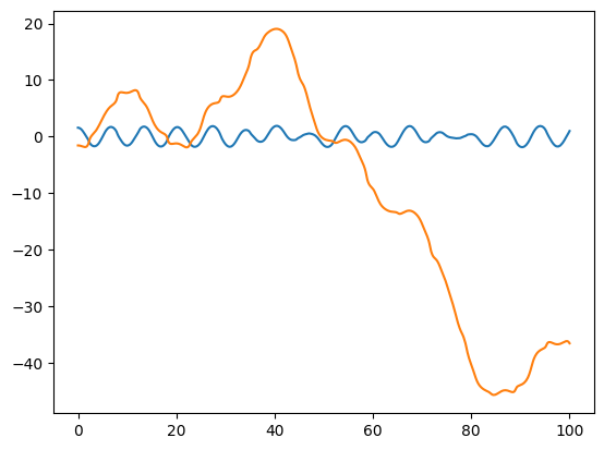
plt.plot(T, X)
[<matplotlib.lines.Line2D at 0x7ff76cb51dc0>,
 <matplotlib.lines.Line2D at 0x7ff76cb51df0>]
# Step 7. Animate the result

from matplotlib import animation
from IPython.display import HTML

fig = plt.figure(figsize=(8,8))
ax  = plt.axes(xlim=(-2.5, 2.5), ylim=(-2.5, 2.5))
ax.set_aspect('equal')

line, = ax.plot([], [], 'o-', lw=2)

def init():
    line.set_data([], [])
    return line,

def animate(i):
    th1 = X[i,0]
    th2 = X[i,1]

    x1 =   np.sin(th1)
    y1 = - np.cos(th1)

    x2 =   np.sin(th2)
    y2 = - np.cos(th2)

    line.set_data([0, x1, x1+x2], [0, y1, y1+y2])
    return line,

anim = animation.FuncAnimation(fig, animate, init_func=init, frames=len(T), interval=20, blit=True)

plt.close()

HTML(anim.to_html5_video())
---------------------------------------------------------------------------
RuntimeError                              Traceback (most recent call last)
Cell In[10], line 33
     29 anim = animation.FuncAnimation(fig, animate, init_func=init, frames=len(T), interval=20, blit=True)
     31 plt.close()
---> 33 HTML(anim.to_html5_video())

File /opt/hostedtoolcache/Python/3.12.10/x64/lib/python3.12/site-packages/matplotlib/animation.py:1302, in Animation.to_html5_video(self, embed_limit)
   1299 path = Path(tmpdir, "temp.m4v")
   1300 # We create a writer manually so that we can get the
   1301 # appropriate size for the tag
-> 1302 Writer = writers[mpl.rcParams['animation.writer']]
   1303 writer = Writer(codec='h264',
   1304                 bitrate=mpl.rcParams['animation.bitrate'],
   1305                 fps=1000. / self._interval)
   1306 self.save(str(path), writer=writer)

File /opt/hostedtoolcache/Python/3.12.10/x64/lib/python3.12/site-packages/matplotlib/animation.py:121, in MovieWriterRegistry.__getitem__(self, name)
    119 if self.is_available(name):
    120     return self._registered[name]
--> 121 raise RuntimeError(f"Requested MovieWriter ({name}) not available")

RuntimeError: Requested MovieWriter (ffmpeg) not available