Integration Lab#
In this lab, you will explore two important challenges in numerical integration:
Handling improper integrals using coordinate transformation. Many real-world integrals have infinite limits or singularities. Direct numerical integration often fails, so we apply variable transformations to map the integral to a finite domain.
Investigating convergence properties for functions with discontinuities. Standard numerical methods assume smoothness for high accuracy. If the function has a jump discontinuity, we will observe how the convergence rate deteriorates.
Handling an Improper Integral via Coordinate Transformation#
Consider the improper integral:
This integral is well-known, and its exact value is:
However, standard numerical integration methods fail because the domain extends to infinity. To solve this, we introduce a coordinate transformation that maps the infinite domain \([0, \infty)\) to a finite domain \([0,1]\).
Coordinate Transformation#
A common transformation is:
Differentiating,
Rewriting the integral in terms of \(t\):
This transforms the infinite limit \(x = \infty\) to the finite limit \(t = 1\), allowing us to apply numerical integration techniques.
import numpy as np
from matplotlib import pyplot as plt
# HANDSON: Define the original function
def f(x):
    return 1 / (1 + x**2)
# HANDSON: Define the transformed function
def ft(t):
    x  = t / (1 - t)    # Change of variable
    xd = 1 / (1 - t)**2 # Derivative $\dot{x} = dx/dt$
    return f(x) * xd
# HANDSON: Implement Middle Riemann Sum
def middle(f, N, a=0, b=1):
    h = (b - a) / N
    x = a + (np.arange(N) + 0.5) * h
    return np.sum(f(x)) * h
# Perform the integration using the transformed variable
N = 64  # Number of sub-intervals
I = np.pi / 2
I_middle = middle(ft, N)
#I_test   = middle(ft,

# Print results
print(f"Middle Riemann Sum (N={N}): {I_middle}")
print(f"Exact Integral: {I}")
print(f"Absolute Error: {abs(I_middle - I)}")
Middle Riemann Sum (N=64): 1.5708370168981682
Exact Integral: 1.5707963267948966
Absolute Error: 4.069010327167888e-05
Integrating a Function with a Jump Discontinuity#
Many numerical integration methods assume smoothness of the function. However, when the function has a jump discontinuity, the convergence rate degrades significantly.
Consider the function:
We compute the definite integral:
Since the function is piecewise constant, the exact integral is \(2/\pi + 1/2\). However, standard numerical integration methods will struggle to approximate this accurately due to the jump at \(x = 0.5\).
# HANDSON: Define the left and right functions
def fL(x):
    return np.sin(np.pi * x)

def fR(x):
    return np.sin(np.pi * x) + 1

def f(x):
    return np.where(x < 0.5, fL(x), fR(x))
# HANDSON: Implement the Trapezoidal Rule
def trapezoidal(f, N=8, a=0, b=1):
    X, D = np.linspace(a, b, N+1, retstep=True)
    return np.sum(f(X[1:]) + f(X[:-1])) * 0.5 * D
# HANDSON: Implement Simpson's Rule
def simpson(f, N=8, a=0, b=1):
    X, D = np.linspace(a, b, N+1, retstep=True)
    S = 0
    for i in range(N // 2):
        l = X[2 * i]
        m = X[2 * i + 1]
        r = X[2 * i + 2]
        S += D * (f(l) + 4 * f(m) + f(r)) / 3
    return S
# Compute exact integral
I = 2/np.pi + 0.5

# Compare convergence for different methods
Ns = [4, 8, 16, 32, 64, 128, 256]
errs_trap  = []
errs_simp  = []
errs_trap2 = []
errs_simp2 = []

for N in Ns:
    I_trap  = trapezoidal(f, N)
    I_simp  = simpson    (f, N)
    I_trap2 = trapezoidal(fL, N//2, 0, 0.5) + trapezoidal(fR, N//2, 0.5, 1)
    I_simp2 = simpson    (fL, N//2, 0, 0.5) + simpson    (fR, N//2, 0.5, 1)
    errs_trap .append(abs(I_trap  - I))
    errs_simp .append(abs(I_simp  - I))
    errs_trap2.append(abs(I_trap2 - I))
    errs_simp2.append(abs(I_simp2 - I))

# Plot error convergence
plt.loglog(Ns, errs_trap,  'o--', label='Trapezoidal Rule')
plt.loglog(Ns, errs_simp,  's--', label='Simpson’s Rule')
plt.loglog(Ns, errs_trap2, 'o-',  label='Trapezoidal Rule 2')
plt.loglog(Ns, errs_simp2, 's-',  label='Simpson’s Rule 2')
plt.loglog(Ns, np.array(Ns)**(-1.), ':', label=r'$N^{-1}$ reference')
plt.loglog(Ns, np.array(Ns)**(-2.), ':', label=r'$N^{-2}$ reference')
plt.xlabel('Number of Intervals (N)')
plt.ylabel('Absolute Error')
plt.legend()
plt.title('Convergence of Numerical Integration on a Discontinuous Function')
plt.show()
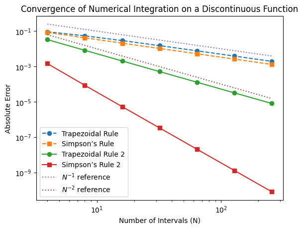
Observations
Degraded Convergence Rate
For smooth functions, Simpson’s rule is expected to converge at \(\mathcal{O}(N^{-4})\).
However, due to the discontinuity at \(x = 0.5\), it instead converges at \(\mathcal{O}(N^{-1})\).
Poor Accuracy for Large (N)
Increasing (N) does not always help significantly because the integration points do not align with the discontinuity.
Potential Fixes
Refinement Near the Discontinuity: Placing additional points near \(x = 0.5\) (which we didn’t implement).
Splitting the Integral: Compute separate integrals for \([0, 0.5]\) and \([0.5, 1]\).