Projectile Motion Lab

In elementary physics courses, one often sees the projectile motion problem without air resistance, for which the solution is fully analytic and straightforward:

• The maximum range occurs at a \(45^\circ\) launch angle,

• The horizontal range is given by the well-known formula \(R = (v_0^2/g) \sin(2\theta)\).

However, if we include air resistance, the situation becomes more complicated.

This lab shows:

1. No Air Resistance: Simple closed-form solution and a quick check via gradient descent.

2. Linear Air Resistance: An analytic solution for \(x(t)\) and \(y(t)\) is still possible, although the time-of-flight can only be solved implicitly (involving a transcendental equation). We can still implement a gradient descent on the angle \(\alpha\), using these closed-form expressions plus a (small) numerical step to find the time of flight.

Gradient Descent for Maximum Range (No Air Resistance)

We consider a projectile launched from the ground at an initial speed \(v_0\) and an angle \(\theta\) with respect to the horizontal. The only force acting on the projectile is gravity, which causes a uniform downward acceleration \(g\). The motion can be decomposed into horizontal and vertical components.

(220)\[\begin{align} \frac{dx}{dt} = v_x, &\quad \frac{dy}{dt} = v_y; \\ \frac{dv_x}{dt} = 0, &\quad \frac{dv_y}{dt} = -g. \end{align}\]

The solution can be obtained by the kinematic equations:

(221)\[\begin{align} x &= v_0\cos(\theta)\;t, \\ y &= v_0\sin(\theta)\;t - \frac{1}{2}gt^2. \end{align}\]

where we chose \(x(t=0) = 0\) and \(y(t=0) = 0\).

The time of flight is simply the non-trivial root of \(y(t)\), which has the analytical form

(222)\[\begin{align} T = \frac{2 v_0 \sin(\theta)}{g}. \end{align}\]

Substituting this into \(x(t)\), the horizontal range is

(223)\[\begin{align} R = x(T) = 2\frac{v_0^2}{g}\sin(\theta)\cos(\theta). \end{align}\]

Using the double angle identities \(\sin(2\theta) \equiv 2\sin(\theta)\cos(\theta)\), we obtain the horizontal range equation

(224)\[\begin{align} R(\theta) = \frac{v_0^2}{g}\sin(2\theta) \end{align}\]

Holding \(v_0\) and \(g\) fix, clearly, \(R(\theta)\) reaches the longest range at \(\sin\)’s peak, i.e., \(2\theta = \pi/2\). This is nothing but the well known result that the maximum range occurs at a \(\theta = \pi/4 = 45^\circ\) launch angle.

In this part of the lab, we will use gradient descent to confirm this numerically.

Task 1: Implement the Range Function

The horizontal range of a projectile launched at an angle \(\theta\) is:

(225)\[\begin{align} R(\theta) = \frac{v_0^2}{g} \sin(2\theta). \end{align}\]

Define a Python function R_proj(theta, v0, g) that computes \(R(\theta)\).

# HANDSON: Implement the range equation

from jax import numpy as np

def R_proj(theta, v0, g):
    return (v0*v0 / g) * np.sin(2 * theta)

# HANDSON: implement autodg_hist() with early stop that checks `abs(X[-1] - X[-2]) < tol`

from jax import grad

def autogd_hist(f, x, alpha, imax=1000, tol=1e-6):
    df = grad(f)
    X  = [x]
    for _ in range(imax):
        X.append(X[-1] - alpha * df(X[-1]))
        if abs(X[-1] - X[-2]) < tol:
            break
    return X

import matplotlib.pyplot as plt

# Parameters
v0 = 10    # Initial velocity (m/s)
g  = 9.81  # Gravity (m/s^2)

# Gradient Descent Optimization
theta = np.radians(30)  # Initial guess (in radians)
alpha = 0.01            # Learning rate

# HANSON: Define a loss function L(theta) based on R_proj but depends only on theta
f = lambda alpha: -R_proj(alpha, v0, g)

# HANSON: Use autograd_hist() to obtain the history of Theta
Theta = autogd_hist(f, theta, alpha)

# Convert results to degrees
Theta_deg = np.degrees(np.array(Theta))

# Print result
print(f"Optimized launch angle (degrees): {Theta_deg[-1]}")

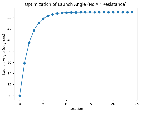
Optimized launch angle (degrees): 44.99994659423828

# Plot results

plt.plot(Theta_deg, '-o')
plt.title('Optimization of Launch Angle (No Air Resistance)')
plt.xlabel('Iteration')
plt.ylabel('Launch Angle (degrees)')

Text(0, 0.5, 'Launch Angle (degrees)')

Gradient Descent for Maximum Range with Air Resistance

When air resistance is included, the force acting on the projectile consists of two components:

• Gravity: \(- mg\hat{j}\)

• Air Resistance: \(-k\mathbf{v}\), where \(k\) is the drag coefficient and \(\mathbf{v} = (v_x, v_y)\) is the velocity.

Defining \(\gamma = k/m\) as the damping coefficient, Newton’s second law gives the system of differential equations:

(226)\[\begin{align} \frac{d v_x}{dt} &= - \gamma v_x, \\ \frac{d v_y}{dt} &= -g - \gamma v_y. \end{align}\]

The first equation is a simple separable differential equation. Integrating both sides and using the initial condition \(v_x(0) = v_0 \cos(\theta)\),

(227)\[\begin{align} v_x(t) = v_0 \cos(\theta)\,e^{-\gamma t}. \end{align}\]

Using the integrating factor method, the general solution to the second equation is

(228)\[\begin{align} v_y = e^{-\gamma t} \left( C - \int g e^{\gamma t} dt \right). \end{align}\]

Solving the integral and using the initial condition \(v_y(0) = v_0 \sin(\theta)\), we have

(229)\[\begin{align} v_y(t) = \left( v_0 \sin\theta + \frac{g}{\gamma} \right) e^{-\gamma t} - \frac{g}{\gamma} \end{align}\]

Note that \(v_\text{t} \equiv g/\gamma\) is the terminating velocity. Hence the vertical equation can be rewritten as:

(230)\[\begin{align} v_y(t) = v_0 \sin(\theta)\;e^{-\gamma t} - v_\text{t}(1 - e^{-\gamma t}). \end{align}\]

Integrating \(v_x(t)\) and \(v_y(t)\) in time, we obtain the complicated but still analytical equations

(231)\[\begin{align} x(t) &= \frac{v_0 \cos\theta}{\gamma} \left( 1 - e^{-\gamma t} \right)\\ y(t) &= \frac{v_0 \sin\theta + v_\text{t}}{\gamma} \left(1 - e^{-\gamma t} \right) - v_\text{t} t. \end{align}\]

The flight of time in this case, i.e., the non-trivial root of \(y(t)\) does not have an analytical solution. While it is possible to use a root finder to solve it numerically, for this hands-on lab, we will make a simplification.

Event without air resistance, i.e., when \(\gamma = 0\), the flight of time at 0 air resistance \(T_0\) is finite. Hence, we can consider the situation that \(\gamma \ll 1 / T_0\). This allows us to Taylor expansion the horizontal equation

(232)\[\begin{align} y(t) &\approx \frac{v_0 \sin\theta + v_\text{t}}{\gamma} \left(\gamma t - \frac{\gamma^2 t^2}{2}\right) - v_\text{t} t \\ &= v_0 \sin(\theta)\;t - \frac{\gamma v_0\sin\theta + g}{2}\;t^2. \end{align}\]

Hence, the corrected flight of time at small air resistance is

(233)\[\begin{align} T_\gamma \approx \frac{2v_0\sin\theta}{\gamma v_0\sin\theta + g}. \end{align}\]

Keeping the horizontal equation at the same order and substitute the flight of time, we have

(234)\[\begin{align} R = x(T_\gamma) \approx v_0\cos(\theta) T_\gamma \approx \frac{v_0^2\sin 2\theta}{\gamma v_0\sin\theta + g}. \end{align}\]

Holding \(v_0\), \(g\), and \(\gamma\) fix, we can find the longest range by maximizing:

(235)\[\begin{align} R(\theta) \approx \frac{v_0^2\sin 2\theta}{\gamma v_0\sin\theta + g}. \end{align}\]

# HANDSON: Implement flight of time

def T_flight(theta, v0, g, gamma=0):
    vy = v0 * np.sin(theta)
    return 2 * vy / (gamma * vy + g)

# HANDSON: Implement the range equation

def R_proj(theta, v0, g, gamma=0):
    return v0*v0 * np.sin(2 * theta) / (gamma * v0 * np.sin(theta) + g)

# Parameters
v0    = 10    # Initial velocity (m/s)
g     = 9.8   # Gravity (m/s^2)
gamma = 0.01  # Damping coefficient (1/s)

# Gradient Descent Optimization
theta = np.radians(30)  # Initial guess (in radians)
alpha = 0.01            # Learning rate

# HANSON: Define a loss function L(theta) based on R_proj but depends only on theta
f = lambda theta: -R_proj(theta, v0, g, gamma)

# HANSON: Use autograd_hist() to obtain the history of Theta
Theta = autogd_hist(f, theta, alpha, imax=50)

# HANDSON: use T_flight() to check if we expect a good approximation

T = T_flight(Theta[-1], v0, g, gamma)
print("gamma:", gamma)
print("T_flight:", T)
print("gamma * T_flight:", gamma * T)

if gamma * T < 0.1:
    print("Good approximation :-)")
else:
    print("Bad approximation  :-(")

gamma: 0.01
T_flight: 1.4301814
gamma * T_flight: 0.014301813
Good approximation :-)

# Convert results to degrees
Theta_deg = np.degrees(np.array(Theta))

# Print result
print(f"Optimized launch angle (degrees): {Theta_deg[-1]}")
print(f"{Theta[-1]}")

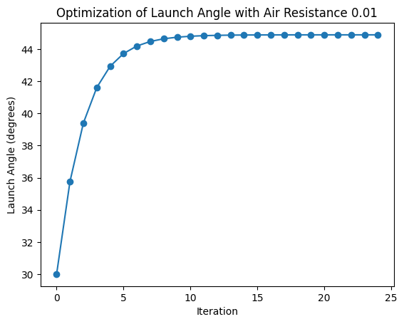
Optimized launch angle (degrees): 44.89714431762695
0.7836029529571533

# Plot results

plt.plot(Theta_deg, '-o')
plt.title(f'Optimization of Launch Angle with Air Resistance {gamma}')
plt.xlabel('Iteration')
plt.ylabel('Launch Angle (degrees)')

Text(0, 0.5, 'Launch Angle (degrees)')