ODE Lab I: 4th-order Runge-Kutta Methods

In this lab, we will study two different 4th-order Runge-Kutta (RK) methods and compare their performance on a simple test problem: the simple harmonic oscillator. We will:

1. Review the classical RK4 method.

2. Implement both the classical RK4 and the 3/8 method of Kutta (1901).

3. Compare their numerical errors and observe the expected 4th-order convergence.

Background

The Classical RK4 Method

You have already seen in lecture that the 4th-order Runge-Kutta (RK4) method is a widely used time-integration scheme for ordinary differential equations (ODEs) of the form

(347)\[\begin{align} \frac{dX}{dt} = f(X, t), \quad X(t_0) = X_0. \end{align}\]

At each step, we compute four “slopes”:

(348)\[\begin{align} k_1 &= \Delta t \, f(X_n, t_n) \\ k_2 &= \Delta t \, f\left(X_n + \frac{1}{2}k_1, t_n + \frac{1}{2}\Delta t\right) \\ k_3 &= \Delta t \, f\left(X_n + \frac{1}{2}k_2, t_n + \frac{1}{2}\Delta t\right) \\ k_4 &= \Delta t \, f\left(X_n + k_3, t_n + \Delta t\right) \end{align}\]

Then we update X_{n+1} according to:

(349)\[\begin{align} X_{n+1} = X_n + \frac{1}{6} k_1 + \frac{1}{3} k_2 + \frac{1}{3} k_3 + \frac{1}{6} k_4. \end{align}\]

This scheme is fourth-order accurate, meaning the local truncation error is \(\mathcal{O}(\Delta t^5)\), and the global error (error over an entire integration interval) behaves like \(\mathcal{O}(\Delta t^4)\).

The “3/8” Method (Kutta, 1901)

An alternative set of coefficients yielding the same order of accuracy is:

(350)\[\begin{align} k_1 &= \Delta t \, f(X_n, t_n) \\ k_2 &= \Delta t \, f\left(X_n + \frac{1}{3}k_1, t_n + \frac{1}{3}\Delta t\right) \\ k_3 &= \Delta t \, f\left(X_n + k_2 - \frac{1}{3}k_1, t_n + \frac{2}{3}\Delta t\right) \\ k_4 &= \Delta t \, f\left(X_n + k_3 - k_2 + k_1, t_n + \Delta t\right) \end{align}\]

with

(351)\[\begin{align} X_{n+1} = X_n + \frac{1}{8} k_1 + \frac{3}{8} k_2 + \frac{3}{8} k_3 + \frac{1}{8} k_4. \end{align}\]

Again, this achieves fourth-order global accuracy despite having different coefficients than the more common RK4 method.

Implementing the Methods in Python

Below, you will find two Python functions: RK4() for the classical method, and RK38() for the 3/8 method. Both integrate an ODE

(352)\[\begin{align} \frac{d}{dt} \begin{pmatrix} x_1 \\ x_2 \\ \vdots \end{pmatrix} = f\bigl(x_1, x_2, \ldots, t\bigr), \end{align}\]

over \(n\) steps, starting from an initial state \(X\) at time \(t\), with time step \(dt\).

import numpy as np
from matplotlib import pyplot as plt

def RK4(f, x, t, dt, n):
    """
    Integrate an ODE using the classical RK4 method.
    
    Parameters
    ----------
    f : function
        The function f(x1, x2, ..., t) returning the derivative(s).
    x : np.ndarray
        The initial condition (can be scalar or vector).
    t : float
        The initial time.
    dt : float
        The time step.
    n : int
        Number of steps to take.
    
    Returns
    -------
    T : np.ndarray
        Times at each integration step, of length n+1.
    X : np.ndarray
        Approximate solutions at each step, shape (n+1, len(x)).
    """
    T = np.array(t)
    X = np.array(x)

    for i in range(n):
        k1 = dt * np.array(f(*(x         )))
        k2 = dt * np.array(f(*(x + 0.5*k1)))
        k3 = dt * np.array(f(*(x + 0.5*k2)))
        k4 = dt * np.array(f(*(x +     k3)))

        t += dt
        x += k1/6 + k2/3 + k3/3 + k4/6

        T = np.append( T, t)
        X = np.vstack((X, x))

    return T, X

def RK38(f, x, t, dt, n):
    """
    Integrate an ODE using the 3/8 RK method (Kutta, 1901).
    
    Parameters
    ----------
    f : function
        The function f(x1, x2, ..., t) returning the derivative(s).
    x : np.ndarray
        The initial condition (can be scalar or vector).
    t : float
        The initial time.
    dt : float
        The time step.
    n : int
        Number of steps to take.
    
    Returns
    -------
    T : np.ndarray
        Times at each integration step, of length n+1.
    X : np.ndarray
        Approximate solutions at each step, shape (n+1, len(x)).
    """
    T = np.array(t)
    X = np.array(x)

    for i in range(n):
        k1 = dt * np.array(f(*(x             )))
        k2 = dt * np.array(f(*(x +       k1/3)))
        k3 = dt * np.array(f(*(x +    k2-k1/3)))
        k4 = dt * np.array(f(*(x + k3-k2+k1  )))

        t += dt
        x += (k1 + 3*k2 + 3*k3 + k4)/8

        T = np.append( T, t)
        X = np.vstack((X, x))

    return T, X

Test Problem: Simple Harmonic Oscillator

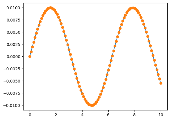
We will use the simple harmonic oscillator with small initial amplitude as our test ODE. Let

(353)\[\begin{align} \frac{d\theta}{dt} = \omega, \quad \frac{d\omega}{dt} = -\theta. \end{align}\]

If we start with \(\theta(0) = 0\) and \(\omega(0) = 0.01\), the exact solution is

(354)\[\begin{align} \theta(t) = 0.01 \sin(t), \quad \omega(t) = 0.01 \cos(t). \end{align}\]

def f_sh(theta, omega):
    """
    Returns the RHS of the simple harmonic oscillator.
    dtheta/dt = omega
    domega/dt = -theta
    """
    return omega, -theta

T, X = RK4(f_sh, (0, 0.01), 0, 0.1, 100)

Theta = X[:,0]
Omega = X[:,1]

plt.plot(T, 0.01*np.sin(T))
plt.plot(T, Theta, 'o')

[<matplotlib.lines.Line2D at 0x7f51eb368fb0>]

Measuring the Error

For a given number of steps \(N\) over a fixed time interval \(t \in [0, T_{\max}]\), we have a time step \(\Delta t = T_\max/N\). After computing the solution numerically, we compare it to the exact solution

(355)\[\begin{align} \theta_\text{exact}(t_i) = 0.01 \sin(t_i). \end{align}\]

We will measure the maximum absolute error in \(\theta\) (though you could also compare \(\omega\)):

(356)\[\begin{align} \text{error} = \max_i \Bigl|\theta_\text{numeric}(t_i) - \theta_\text{exact}(t_i)\Bigr|. \end{align}\]

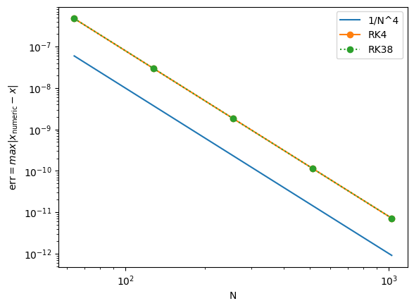
We expect 4th-order methods to show an error scaling like \(\mathcal{O}(\Delta t^4)\), so plotting on a log-log scale should reveal a slope of about -4.

1. Defines a function error_RK4(N) that runs RK4() with N steps and returns the maximum error in \(\theta\).

2. Similarly defines error_RK38(N) for the 3/8 method.

3. Compares both over a range of N values (e.g., 64, 128, 256, 512, 1024).

4. Plots the results on a log-log scale, together with a reference line \(\propto N^{-4}\).

def error_RK4(N=100):
    T, X = RK4(f_sh, (0, 0.01), 0, 10/N, N)
    Theta  = X[:,0]
    Thetap = 0.01 * np.sin(T)
    return np.max(abs(Theta - Thetap))

def error_RK38(N=100):
    T, X = RK38(f_sh, (0, 0.01), 0, 10/N, N)
    Theta  = X[:,0]
    Thetap = 0.01 * np.sin(T)
    return np.max(abs(Theta - Thetap))

N     = np.array([64, 128, 256, 512, 1024])
ERK4  = np.array([error_RK4(n)  for n in N])
ERK38 = np.array([error_RK38(n) for n in N])

plt.loglog(N, 1/N**4,      label='1/N^4')
plt.loglog(N, ERK4,  'o-', label='RK4')
plt.loglog(N, ERK38, 'o:', label='RK38')
plt.xlabel('N')
plt.ylabel(r'$\text{err} = max|x_\text{numeric} - x|$')
plt.legend()

<matplotlib.legend.Legend at 0x7f51eb3cd190>