Numerical Partial Differential Equation I: Introduction#
Introduction to Partial Differential Equations (PDEs)#
Partial Differential Equations (PDEs) are fundamental tools in the mathematical modeling of various physical phenomena. Unlike Ordinary Differential Equations (ODEs), which involve functions of a single variable and their derivatives, PDEs involve functions of multiple variables and their partial derivatives. This distinction makes PDEs particularly powerful in describing systems where changes occur in more than one dimension, such as in space and time.
What are PDEs?#
A Partial Differential Equation is an equation that relates the partial derivatives of a multivariable function. In general form, a PDE can be written as:
where \(u = u(x_1, x_2, \ldots, x_n)\) is the unknown function, and \(\partial u/\partial x_i\) denotes the partial derivatives of \(u\) with respect to the variables \(x_i\).
PDEs are essential in modeling continuous systems where the state of the system depends on multiple variables. They appear in various fields such as physics, engineering, finance, and biology, describing phenomena like heat conduction, wave propagation, fluid dynamics, and quantum mechanics.
Definition and Significance in Modeling Continuous Systems#
PDEs provide a framework for formulating problems involving functions of several variables and their rates of change. They are indispensable in describing the behavior of physical systems where spatial and temporal variations are intrinsic. For instance:
Heat Equation: Models the distribution of heat (or temperature) in a given region over time.
(478)#\[\begin{align} \frac{\partial u}{\partial t} = \alpha \nabla^2 u \end{align}\]Wave Equation: Describes the propagation of waves, such as sound or electromagnetic waves, through a medium.
(479)#\[\begin{align} \frac{\partial^2 u}{\partial t^2} = c^2 \nabla^2 u \end{align}\]
Laplace’s Equation: Represents steady-state solutions where the system does not change over time, such as electric potential in a region devoid of charge.
(480)#\[\begin{align} \nabla^2 u = 0 \end{align}\]
The ability to model such diverse phenomena underscores the versatility and importance of PDEs in scientific and engineering disciplines.
Contrast with Ordinary Differential Equations (ODEs)#
While both PDEs and ODEs involve differential operators, the key difference lies in the number of independent variables involved:
ODEs: Involve functions of a single independent variable and their derivatives. They are typically used to model systems with dynamics that evolve over time without spatial variation. For example, the simple harmonic oscillator is described by the ODE:
(481)#\[\begin{align} \frac{d^2 x}{dt^2} + \omega^2 x = 0 \end{align}\]PDEs: Involve functions of multiple independent variables and their partial derivatives. They are used to model systems where changes occur across multiple dimensions, such as space and time. For example, the Navier-Stokes equations, which govern fluid flow, are a set of PDEs:
(482)#\[\begin{align} \rho \left( \frac{\partial \mathbf{u}}{\partial t} + (\mathbf{u} \cdot \nabla) \mathbf{u} \right) = -\nabla p + \mu \nabla^2 \mathbf{u} + \mathbf{f} \end{align}\]where \(\mathbf{u}\) is the velocity field, \(p\) is the pressure, \(\rho\) is the density, \(\mu\) is the dynamic viscosity, and \(\mathbf{f}\) represents body forces.
Application in Astrophysical Fluid Systems#
PDEs play a pivotal role in modeling complex astrophysical phenomena, particularly those involving fluid dynamics. Astrophysical fluid systems, such as stellar interiors, accretion disks around black holes, and interstellar gas clouds, exhibit intricate behaviors governed by the laws of fluid mechanics and thermodynamics.
For example, the Euler Equations for inviscid flow and the Magnetohydrodynamic (MHD) Equations for conducting fluids are essential in understanding phenomena like solar flares and the dynamics of the interstellar medium. These equations are inherently PDEs due to the multi-dimensional and time-dependent nature of the systems they describe.
Consider the modeling of stellar convection, where hot plasma rises and cooler plasma sinks within a star’s interior. This process is governed by the Navier-Stokes equations coupled with the heat equation, forming a system of PDEs that describe the velocity field, temperature distribution, and pressure variations within the star.
Furthermore, gravitational waves, ripples in spacetime caused by massive astrophysical events like neutron star mergers, are described by the Einstein Field Equations, which are a set of nonlinear PDEs. Solving these equations numerically requires sophisticated techniques due to their complexity and the need for high precision in predictions.
In summary, PDEs are indispensable in astrophysics for modeling and understanding the dynamic and multifaceted nature of celestial phenomena. The ability to solve these equations, either analytically or numerically, provides deep insights into the behavior and evolution of the universe.
Derivation of Fluid Dynamics Equations#
Understanding the fundamental equations that govern fluid motion is essential for both theoretical studies and practical applications in engineering and astrophysics. This section delves into the derivation of the primary fluid dynamics equations—namely, the Continuity, Momentum (Navier-Stokes), and Energy equations—using the integral forms of conservation laws and applying Green’s and Stokes’ theorems. Additionally, we explore an alternative derivation from the Boltzmann Equation using the Moment Method, providing a comprehensive foundation for modeling fluid behavior in various contexts, including complex astrophysical systems.
Integral Forms of Conservation Laws#
Fluid dynamics is fundamentally rooted in the principles of conservation of mass, momentum, and energy. These principles can be expressed in their integral forms, which consider the behavior of fluid quantities within a finite control volume.
Conservation of Mass (Continuity Equation):
The integral form of the continuity equation states that the rate of change of mass within a control volume \(V\) is equal to the net mass flux entering or leaving the volume through its boundary \(\partial V\):
(483)#\[\begin{align} \frac{d}{dt} \int_V \rho \, dV + \oint_{\partial V} \rho \mathbf{u} \cdot \mathbf{n} \, dS = 0 \end{align}\]where:
\(\rho\) is the fluid density,
\(\mathbf{u}\) is the velocity field,
\(\mathbf{n}\) is the outward-pointing unit normal vector on \(\partial V\).
Conservation of Momentum (Navier-Stokes Equations):
The integral form of the momentum conservation law accounts for the forces acting on the fluid within the control volume. It can be expressed as:
(484)#\[\begin{align} \frac{d}{dt} \int_V \rho \mathbf{u} \, dV + \oint_{\partial V} \rho \mathbf{u} (\mathbf{u} \cdot \mathbf{n}) \, dS = \oint_{\partial V} \mathbf{\Pi} \cdot \mathbf{n} \, dS + \int_V \rho \mathbf{f} \, dV \end{align}\]where:
\(\mathbf{\Pi}\) is the stress tensor,
\(\mathbf{f}\) represents body forces (e.g., gravity).
Conservation of Energy:
The integral form of the energy conservation law relates the rate of change of energy within the control volume to the net energy flux and work done by forces:
(485)#\[\begin{align} \frac{d}{dt} \int_V \rho e \, dV + \oint_{\partial V} \rho e \mathbf{u} \cdot \mathbf{n} \, dS = \oint_{\partial V} \mathbf{q} \cdot \mathbf{n} \, dS + \oint_{\partial V} \mathbf{\Pi} \cdot \mathbf{u} \, dS + \int_V \rho \mathbf{f} \cdot \mathbf{u} \, dV \end{align}\]where:
\(e\) is the specific internal energy,
\(\mathbf{q}\) is the heat flux vector.
From Integral to Differential Forms Using Green’s Theorems#
To transition from the integral to the differential forms of these conservation laws, we employ Green’s theorems, which relate volume integrals to surface integrals.
The Divergence Theorem converts a volume integral of a divergence of a vector field into a surface integral over the boundary of the volume:
Application to Conservation of Mass#
Applying the Divergence Theorem to the continuity equation:
This yields the Continuity Equation in differential form:
Application to Conservation of Momentum#
Applying the Divergence Theorem to the momentum equation:
To obtain the Navier-Stokes Equations, we express the stress tensor \(\mathbf{\Pi}\) for a Newtonian fluid:
where:
\(p\) is the pressure,
\(\mu\) is the dynamic viscosity,
\(\lambda\) is the second coefficient of viscosity,
\(\mathbf{I}\) is the identity tensor.
Substituting \(\mathbf{\Pi}\) into the momentum equation and simplifying under the assumption of incompressible flow (\( \nabla \cdot \mathbf{u} = 0\)) leads to:
Application to Conservation of Energy#
Similarly, applying the Divergence Theorem to the energy equation:
Assuming Fourier’s law for heat conduction (\(\mathbf{q} = -k \nabla T\)) and substituting the expression for \( \mathbf{\Pi}\), we obtain the Energy Equation in differential form:
where \(\Phi\) represents the viscous dissipation function.
Moments of the Boltzmann Equation#
To transition from the kinetic description to a fluid description, we take velocity moments of the Boltzmann equation. Key moments correspond to macroscopic quantities:
Zeroth Moment (Density): The zeroth moment gives the mass density:
(495)#\[\begin{align} \rho = \int f m \, d^3\mathbf{v}, \end{align}\]where \(m\) is the particle mass.
First Moment (Momentum Density): The first moment gives the momentum density:
(496)#\[\begin{align} \rho \mathbf{u} = \int f m \mathbf{v} \, d^3\mathbf{v}, \end{align}\]where \(\mathbf{u}\) is the bulk fluid velocity.
Second Moment (Energy Density and Stress): The second moment gives the energy density and stress tensor:
(497)#\[\begin{align} E = \frac{1}{2} \int f m |\mathbf{v}|^2 \, d^3\mathbf{v}, \end{align}\]and
(498)#\[\begin{align} \mathbf{P} = \int f m (\mathbf{v} - \mathbf{u})(\mathbf{v} - \mathbf{u}) \, d^3\mathbf{v}, \end{align}\]where \(\mathbf{P}\) is the pressure tensor.
These moments form the foundation for deriving the fluid equations.
Deriving the Continuity Equation#
The zeroth moment of the Boltzmann equation yields the continuity equation, which expresses the conservation of mass. Integrating the Boltzmann equation over all velocities and assuming no particle creation or destruction:
Deriving the Momentum Equation#
The first moment of the Boltzmann equation provides the momentum equation, which describes the conservation of momentum. Multiplying the Boltzmann equation by \(\mathbf{v}\) and integrating over all velocities:
where:
\(\mathbf{P}\) is the pressure tensor,
\(\mathbf{F}\) represents external forces (e.g., gravity).
The pressure tensor \(\mathbf{P}\) captures both isotropic and anisotropic contributions to stress. It can be decomposed into:
where:
\(p = \frac{1}{3} \text{Tr}(\mathbf{P})\) is the scalar pressure,
\(\mathbf{I}\) is the identity matrix,
\(\boldsymbol{\tau}\) is the deviatoric stress tensor, representing viscous effects.
The momentum equation becomes:
This equation captures the effects of pressure, viscosity, and external forces on fluid motion.
Deriving the Energy Equation#
The second moment of the Boltzmann equation yields the energy equation, which expresses the conservation of energy. Multiplying the Boltzmann equation by \(m|\mathbf{v}|^2/2\) and integrating over all velocities:
where:
\(E = \rho e + \rho |\mathbf{u}|^2/2\) is the total energy density (internal + kinetic),
\(\mathbf{q} = \int f m (\mathbf{v} - \mathbf{u}) (1/2)|\mathbf{v} - \mathbf{u}|^2 \, d^3\mathbf{v}\) is the heat flux.
The internal energy density \(\rho e\) relates to the scalar pressure \(p\) via the equation of state, typically written as:
where \(\gamma\) is the adiabatic index.
The energy equation can be rewritten to highlight internal energy evolution:
This formulation shows how compression, viscous dissipation, and heat conduction influence internal energy.
Closing the System of Equations#
The derived equations—continuity, momentum, and energy—form a coupled system. However, these equations alone are insufficient because they depend on quantities like pressure, stress, and heat flux, which require additional modeling.
Equation of State (EOS): An equation of state, such as \(p = \rho RT\) for an ideal gas, relates pressure, density, and temperature, providing closure for the scalar pressure \(p\).
Viscous Stress (Constitutive Relations): The deviatoric stress tensor \(\boldsymbol{\tau}\) is often modeled using Newtonian fluid assumptions:
(506)#\[\begin{align} \boldsymbol{\tau} = \mu \left( \nabla \mathbf{u} + (\nabla \mathbf{u})^T - \frac{2}{3}(\nabla \cdot \mathbf{u}) \mathbf{I} \right), \end{align}\]where \(\mu\) is the dynamic viscosity.
Heat Flux: Heat flux \(\mathbf{q}\) can be modeled using Fourier’s law:
(507)#\[\begin{align} \mathbf{q} = -k \nabla T, \end{align}\]where \(k\) is the thermal conductivity.
These closure relations reduce the system to a solvable set of equations.
Assumptions & Physical Meaning#
Several key assumptions underpin the derivation of the Navier-Stokes equations, simplifying the complex interactions within a fluid to make the equations tractable:
Continuum Hypothesis:
Assumes that fluid properties such as density and velocity are continuously distributed in space. This is valid when the mean free path of particles is much smaller than the characteristic length scales of interest.
Newtonian Fluid:
Assumes that the stress tensor \(\mathbf{\Pi}\) is linearly related to the strain rate tensor. This implies that the fluid’s viscosity is constant and that the relationship between shear stress and strain rate is proportional.
Local Thermodynamic Equilibrium:
Assumes that the distribution function \(f\) is close to the Maxwell-Boltzmann distribution, allowing for the expansion of \(f\) in terms of small deviations. This ensures that macroscopic quantities like temperature and pressure are well-defined locally.
Negligible External Forces:
Often, body forces \(\mathbf{f}\) such as gravity are considered constant or negligible compared to other forces. In cases where external forces are significant, they are incorporated explicitly into the momentum and energy equations.
Incompressible Flow:
For many practical applications, especially at low Mach numbers, the fluid is assumed to be incompressible (\(\nabla \cdot \mathbf{u} = 0\)). This simplifies the continuity equation and decouples the pressure from the density.
Viscosity, Pressure Gradients, and Other Key Terms#
Pressure Gradient (\(-\nabla p\)):
Represents the force per unit volume exerted by pressure differences within the fluid. It drives the fluid from regions of high pressure to low pressure, influencing the acceleration and direction of flow.
Viscous Terms (\(\mu \nabla^2 \mathbf{u}\)):
Account for internal friction due to the fluid’s viscosity, which resists deformation and dissipates kinetic energy into thermal energy. Viscosity is a measure of a fluid’s resistance to shear or flow.
Body Forces (\(\rho \mathbf{f}\)):
Represent external forces acting on the fluid, such as gravity or electromagnetic forces. These forces can influence the overall motion and stability of the fluid flow.
These terms collectively describe the balance between inertial forces, pressure forces, viscous forces, and external influences, shaping the fluid’s behavior under various conditions.
Limiting Cases and Their Physical Interpretations#
Analyzing the Navier-Stokes equations under different assumptions and limiting cases provides deeper insights into fluid behavior:
Inviscid Flow (Euler Equations):
By setting viscosity \(\mu = 0\), the Navier-Stokes equations reduce to the Euler equations:
(508)#\[\begin{align} \rho \left( \frac{\partial \mathbf{u}}{\partial t} + (\mathbf{u} \cdot \nabla) \mathbf{u} \right) = -\nabla p + \rho \mathbf{f} \end{align}\]These equations describe ideal, non-viscous fluid flow and are applicable in scenarios where viscous effects are negligible, such as high Reynolds number flows.
Steady-State Flow:
Assuming no temporal changes (\(\frac{\partial}{\partial t} = 0\)), the equations describe steady-state conditions where fluid properties remain constant over time. This simplification is useful in analyzing flows that have reached equilibrium.
Laminar vs. Turbulent Flow:
Laminar Flow: Occurs at low Reynolds numbers where viscous forces dominate, resulting in smooth, orderly fluid motion.
Turbulent Flow: Arises at high Reynolds numbers where inertial forces prevail, leading to chaotic and eddying fluid motion.
Understanding these limiting cases aids in selecting appropriate models and computational approaches for different fluid flow regimes.
Significance in Fluid Dynamics#
The derived fluid dynamics equations, particularly the Navier-Stokes equations, are foundational in describing and predicting fluid behavior across a myriad of applications. Their significance extends from everyday engineering problems to the most complex astrophysical phenomena.
Role of PDEs in Governing Real-World Flows#
Partial Differential Equations (PDEs) like the Navier-Stokes equations encapsulate the fundamental principles governing fluid motion—conservation of mass, momentum, and energy. These equations enable the simulation and analysis of fluid flows in various contexts:
Atmospheric Sciences:
PDEs model weather patterns, climate dynamics, and the movement of air masses, aiding in weather forecasting and climate modeling.
Oceanography:
They describe ocean currents, wave dynamics, and the mixing of different water masses, contributing to the understanding of marine ecosystems and global climate.
Engineering Applications:
In aerospace engineering, PDEs are used to design and optimize aircraft and spacecraft by simulating airflow around structures. In civil engineering, they aid in modeling the flow of water in pipes and channels.
Astrophysics:
PDEs are indispensable for modeling the behavior of astrophysical fluids under extreme conditions, such as those found in stellar interiors, accretion disks, and interstellar gas clouds.
Application in Astrophysical Fluid Systems#
Astrophysical systems often involve complex fluid dynamics under extreme conditions of temperature, pressure, and gravity. PDEs are essential in modeling these systems, providing insights into their structure, evolution, and behavior.
Stellar Interiors:
The interiors of stars involve convective and radiative energy transport, described by the Navier-Stokes equations coupled with the heat equation. These models help in understanding stellar structure, energy generation, and evolution.
Accretion Disks:
Around compact objects like black holes and neutron stars, accretion disks form as matter spirals inward. PDEs model the fluid dynamics, angular momentum transport, and radiation processes within these disks, crucial for explaining phenomena like quasars and X-ray binaries.
Interstellar Medium (ISM):
The ISM consists of gas and dust influenced by gravitational, magnetic, and thermal forces. Magnetohydrodynamic (MHD) equations, a set of PDEs, describe the behavior of conducting fluids in the ISM, aiding in the study of star formation, supernova remnants, and galactic dynamics.
Gravitational Waves:
The propagation of gravitational waves, ripples in spacetime caused by massive astrophysical events, is described by the Einstein Field Equations, which are highly complex nonlinear PDEs. Numerical solutions to these equations are essential for predicting gravitational wave signatures detected by observatories like LIGO and Virgo.
Supernova Explosions:
The explosive death of massive stars involves shock waves, turbulence, and nuclear reactions, all governed by fluid dynamics PDEs. Modeling these processes is crucial for understanding the distribution of heavy elements and the dynamics of supernova remnants.
Classification of Partial Differential Equations (PDEs)#
Partial Differential Equations (PDEs) are integral to modeling a vast array of physical phenomena, from the diffusion of heat to the propagation of waves. Understanding the classification of PDEs is essential for selecting appropriate solution methods and interpreting the behavior of the systems they describe. PDEs are primarily classified into three categories: Elliptic, Parabolic, and Hyperbolic. Each class possesses distinct mathematical properties and governs different types of physical phenomena. This section delves into the nature, applications, and astrophysical relevance of each PDE type.
Elliptic PDEs#
Definition and Characteristics:
Elliptic PDEs are characterized by the absence of real characteristics, implying that the solution at any given point depends on the values of the solution in an entire surrounding region. These equations typically describe steady-state situations where there is no time dependence.
The general second-order linear elliptic PDE in two variables can be written as:
where the discriminant \(B^2 - AC < 0\), ensuring ellipticity.
Example: Laplace’s Equation:
One of the most fundamental elliptic PDEs is Laplace’s equation, given by:
where \(\nabla^2\) is the Laplacian operator. Laplace’s equation arises in various contexts, including electrostatics, gravitational potentials, and incompressible fluid flow.
Physical Intuition and Applications:
Elliptic PDEs model phenomena where the state of the system is in equilibrium. Solutions to elliptic equations are generally smooth and exhibit no abrupt changes, reflecting the steady-state nature of the systems they describe.
Astrophysical Applications:
In astrophysics, Laplace’s equation is used to model gravitational potentials in regions devoid of mass. For instance, the gravitational potential outside a spherically symmetric mass distribution can be described by Laplace’s equation, facilitating the study of stellar and planetary structures.
Parabolic PDEs#
Definition and Characteristics:
Parabolic PDEs are associated with diffusion-like processes and typically involve one temporal dimension and multiple spatial dimensions. They describe how a system evolves over time towards equilibrium.
The general form of a second-order linear parabolic PDE in two variables is:
with the discriminant \(B^2 - 4AC = 0\).
Example: Heat Equation:
The quintessential parabolic PDE is the heat equation:
where \(u\) represents temperature, and \(\alpha\) is the thermal diffusivity of the material.
Physical Intuition and Applications:
Parabolic PDEs model processes where diffusion plays a central role, leading to the smoothing out of gradients over time. Solutions to parabolic equations typically show how an initial distribution evolves, gradually approaching a steady state.
Astrophysical Applications:
In astrophysics, parabolic PDEs are employed to model thermal conduction within stars. For example, the transport of heat from the core to the outer layers of a star can be described by the heat equation, aiding in the understanding of stellar evolution and energy distribution.
Hyperbolic PDEs#
Definition and Characteristics:
Hyperbolic PDEs are associated with wave propagation and are characterized by the existence of real characteristics along which information travels. These equations typically involve both temporal and spatial derivatives and can model dynamic, time-dependent phenomena.
The general form of a second-order linear hyperbolic PDE in two variables is:
where the discriminant \(B^2 - 4AC > 0\), ensuring hyperbolicity.
Example – Wave Equation:
A fundamental example of a hyperbolic PDE is the wave equation:
where \(u\) represents the wave function, and \(c\) is the wave speed.
Physical Intuition and Applications:
Hyperbolic PDEs model systems where disturbances propagate as waves, maintaining their shape over time. Solutions to hyperbolic equations exhibit finite propagation speeds and can describe phenomena such as sound waves, electromagnetic waves, and shock waves.
Astrophysical Applications:
In the astrophysical context, hyperbolic PDEs are essential for modeling wave phenomena in stellar oscillations and the propagation of shock waves in supernova explosions. Additionally, the Einstein Field Equations, which describe gravitational waves in general relativity, are a set of highly nonlinear hyperbolic PDEs.
Physical Intuition Behind Each PDE Type#
Understanding the physical intuition behind each class of PDEs aids in selecting appropriate models and solution techniques for different phenomena:
Elliptic PDEs describe equilibrium states where the system is balanced, and there is no inherent time evolution. They are often used to determine steady-state distributions of physical quantities.
Parabolic PDEs capture the time-dependent evolution of systems towards equilibrium through diffusive processes. They are ideal for modeling heat conduction, mass diffusion, and similar phenomena.
Hyperbolic PDEs represent dynamic systems where disturbances propagate as waves. They are suited for modeling scenarios involving wave motion, vibrations, and other propagating phenomena.
Examples of Physical Phenomena#
Elliptic PDEs:
Electrostatic Potential: Determined by Laplace’s or Poisson’s equation in regions without or with charge distributions, respectively.
Steady-State Fluid Flow: Described by the incompressible Navier-Stokes equations under steady conditions.
Parabolic PDEs:
Heat Conduction: Governed by the heat equation, modeling temperature distribution over time.
Diffusion Processes: Including the spread of pollutants in the atmosphere or solutes in a solvent.
Hyperbolic PDEs:
Sound Waves: Described by the acoustic wave equation, modeling pressure variations in a medium.
Electromagnetic Waves: Governed by Maxwell’s equations, which can be expressed as hyperbolic PDEs.
Gravitational Waves: Modeled by the Einstein Field Equations in the context of general relativity.
Key Dimensionless Numbers#
Several dimensionless numbers play pivotal roles in fluid dynamics and the study of PDEs. Among the most important are the Reynolds Number (Re), Mach Number (Ma), and Prandtl Number (Pr). Each of these numbers encapsulates the ratio of different physical effects, providing insight into the system’s behavior.
Numerical Techniques for Solving PDEs#
Solving Partial Differential Equations (PDEs) numerically is essential for modeling complex physical systems that lack closed-form analytical solutions. Among the various numerical methods available, Finite Difference Methods (FDM) are particularly popular due to their simplicity and ease of implementation. This section delves into the fundamentals of FDM, focusing on the Forward Time Centered Space (FTCS) scheme, and provides a practical Python example for solving the linear advection equation. Subsequent sections will explore stability analysis using Von Neumann methods and introduce stabilized methods to enhance numerical stability.
Finite Difference Methods (FDM)#
Finite Difference Methods approximate the derivatives in PDEs by using difference quotients on a discretized grid. This approach transforms continuous PDEs into discrete algebraic equations that can be solved iteratively. FDM is widely used in engineering and scientific computations due to its straightforward application to regular grids and its compatibility with existing numerical solvers.
Forward Time Centered Space
The Forward Time Centered Space (FTCS) scheme is one of the simplest explicit finite difference methods used to solve time-dependent PDEs. It approximates the time derivative using a forward difference and the spatial derivatives using centered differences. While FTCS is easy to implement, it is conditionally stable, meaning that it requires adherence to specific stability criteria to prevent numerical oscillations and divergence.
Consider the linear advection equation, a fundamental PDE that models the transport of a quantity \(u\) with constant speed \(c\):
Discretization:
Let \(u_i^n\) denote the numerical approximation of \(u\) at spatial index \(i\) and time level \(n\). The FTCS scheme discretizes the advection equation as follows:
Solving for \(u_i^{n+1}\):
This explicit update rule allows the computation of the solution at the next time step based on the current and neighboring spatial points.
import numpy as np
import matplotlib.pyplot as plt
# Parameters
c = 1.0 # Advection speed
L = 1.0 # Domain length
T = 5.0 # Total time
nx = 100 # Number of spatial points
dx = L / nx # Spatial step size
dt = 0.0001 # Initial time step size
nt = int(T / dt) # Number of time steps
# Stability parameter
sigma = c * dt / dx
print(sigma)
# Spatial grid
x = np.linspace(0, L, nx)
u_initial = np.sin(2 * np.pi * x) # Initial condition: sinusoidal wave
# Initialize solution array
u = u_initial.copy()
# Time-stepping loop
for n in range(nt):
# Apply periodic boundary conditions using np.roll
u_new = u - (c * dt / (2 * dx)) * (np.roll(u, -1) - np.roll(u, 1))
u = u_new
# Analytical solution
u_exact = np.sin(2 * np.pi * (x - c * T))
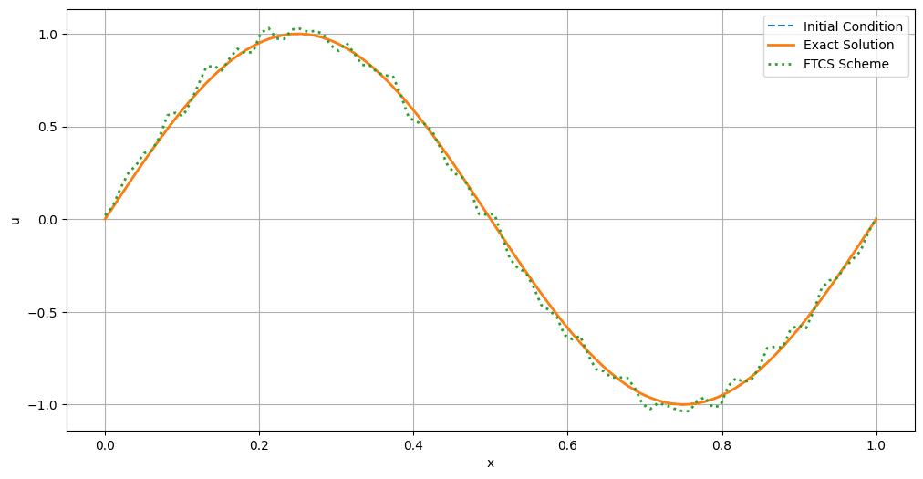
# Plotting the results
plt.figure(figsize=(12, 6))
plt.plot(x, u_initial, label='Initial Condition', linestyle='--')
plt.plot(x, u_exact, label='Exact Solution', linewidth=2)
plt.plot(x, u, label='FTCS Scheme', linestyle=':', linewidth=2)
plt.xlabel('x')
plt.ylabel('u')
plt.legend()
plt.grid(True)
0.01
Inherent Instability Issues#
While the FTCS scheme is straightforward, it is inherently unstable for the linear advection equation unless the time step \(\Delta t\) and spatial step \(\Delta x\) satisfy the Courant-Friedrichs-Lewy (CFL) condition. Failure to adhere to this condition can result in numerical oscillations that grow uncontrollably, leading to divergence of the solution.
By adjusting the time step dt to satisfy the CFL condition, the FTCS scheme produces a stable solution that closely matches the exact analytical solution. If the CFL condition is violated (i.e., \(\sigma > 1\)), the numerical solution becomes unstable, exhibiting oscillations and diverging from the exact solution. This behavior underscores the importance of adhering to stability criteria when applying explicit finite difference schemes like FTCS.
Von Neumann Stability Analysis#
Von Neumann Stability Analysis is a mathematical technique used to assess the stability of finite difference schemes applied to linear partial differential equations (PDEs). This method involves decomposing the numerical solution into Fourier modes and analyzing the growth or decay of these modes over time. If all Fourier modes remain bounded, the numerical scheme is considered stable. Otherwise, the scheme is unstable and may produce erroneous results.
To perform Von Neumann Stability Analysis, we assume a solution of the form:
where:
\(u_i^n\) is the numerical approximation of \(u\) at spatial index \(i\) and time level \(n\).
\(G\) is the amplification factor.
\(k\) is the wave number.
\(x_i = i \Delta x\) is the spatial position of the \(i\)-th grid point.
The goal is to determine whether the magnitude of the amplification factor \(|G|\) remains less than or equal to 1 for all possible wave numbers \(k\). If \(|G| \leq 1\) for all \(k\), the numerical scheme is stable.
Applying Von Neumann Analysis to the FTCS Scheme#
Consider the Forward Time Centered Space (FTCS) scheme applied to the linear advection equation:
FTCS Update Rule:
Assumed Solution:
Substituting into the FTCS Update Rule:
Simplify using \(x_{i \pm 1} = x_i \pm \Delta x\):
Using Euler’s formula \(e^{i\theta} - e^{-i\theta} = 2i \sin(\theta)\):
where \(\sigma = c \Delta t/\Delta x\) is the Courant number.
Calculating the Magnitude of \(G\):
Since \(|G| > 1\) for any \(\sigma > 0\), the FTCS scheme is inherently unstable for the linear advection equation.
In the next lecture, we will provide other (stable) numerical methods to solve the advection equation.