Fourier Transform and Spectral Analyses Lab (Solution)#
Aliasing Errors#
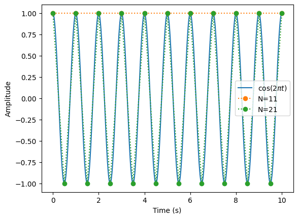
Aliasing occurs when a signal is sampled at a rate insufficient to capture its highest frequency components, causing high-frequency components to appear as lower frequencies. In this section, we will demonstrate aliasing and determine the minimum sampling rate needed to avoid it.
Setup:
Generate a sinusoidal signal \(s(t) = \cos(2\pi t)\).
Sample the signal at different rates and visualize the effect.
from matplotlib import pyplot as plt
import numpy as np
t = np.linspace(0, 10, num=2001) # use very high sampling rate to approximate the analytic function
s = np.cos(2 * np.pi * t) # periodic is 1
plt.plot(t, s, label=r'$\cos(2\pi t)$')

# HANDSON: write a loop to loop over different sampling rates
for N in [11, 21]:
   t = np.linspace(0, 10, num=N)
   s = np.cos(2 * np.pi * t)
   plt.plot(t, s, 'o:', label=f'N={N}')

plt.xlabel('Time (s)')
plt.ylabel('Amplitude')
plt.legend()
<matplotlib.legend.Legend at 0x7f50175354c0>
Spectral Filtering#
Spectral filtering involves transforming a signal into the frequency domain, modifying specific frequency components (e.g., removing noise), and transforming it back to the time domain.
In this section, we will implement a low-pass filter. Setup:
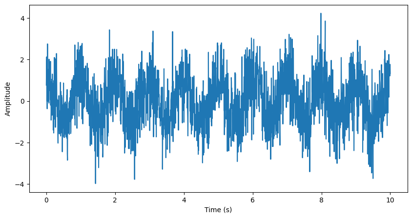
Generate a noisy sinusoidal signal.
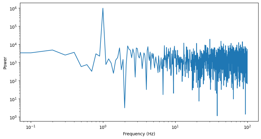
Transform the signal into the frequency domain using the Fast Fourier Transform (FFT).
Apply a low-pass filter to remove high-frequency noise.
Transform the filtered signal back to the time domain.
t = np.linspace(0, 10, num=2000) # use very high sampling rate to approximate the analytic function
s = np.cos(2 * np.pi * t) # periodic is 1

# Add noise
noisy = s + np.random.normal(size=t.shape)

# Visualize the signal with noise
plt.figure(figsize=(10, 5))
plt.plot(t, noisy)
plt.xlabel('Time (s)')
plt.ylabel('Amplitude')
Text(0, 0.5, 'Amplitude')
# Fourier Transform
f = np.fft.fftfreq(len(t), d=t[1])
Noisy = np.fft.fft(noisy)
Power = abs(Noisy[:len(t)//2])**2

plt.figure(figsize=(10, 5))
plt.loglog(f[:len(t)//2], Power)
plt.xlabel('Frequency (Hz)')
plt.ylabel('Power')
Text(0, 0.5, 'Power')
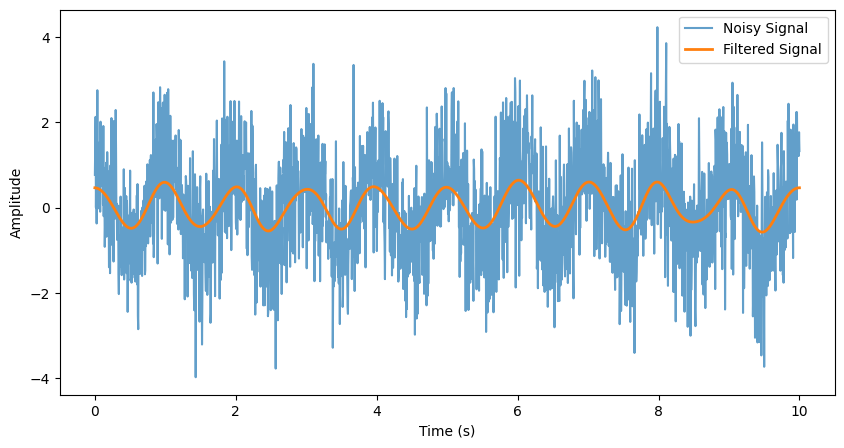
# HANDSON: implement a low pass filter
Noisy[20:] = 0

# and inverse Fourier transform
filtered = np.real(np.fft.ifft(Noisy))
plt.figure(figsize=(10, 5))
plt.plot(t, noisy, label='Noisy Signal', alpha=0.7)
if filtered is not ...:
    plt.plot(t, filtered, label='Filtered Signal', linewidth=2)
plt.xlabel('Time (s)')
plt.ylabel('Amplitude')
plt.legend()
<matplotlib.legend.Legend at 0x7f50175a1d90>