ODE Lab II: Central Potential Problem

In this lab, we will implement two numerical integration methods—Runge-Kutta 4th order (RK4) and Leapfrog/Verlet—to study a 2D central potential problem. This problem models a body in an inverse-square law force field, such as planetary motion under Newtonian gravity.

The equation governing motion in a central potential is:

(409)\[\begin{align} \frac{d^2 \mathbf{r}}{dt^2} = \mathbf{a} = - \nabla \frac{1}{|\mathbf{r}|} = - \frac{\mathbf{r}}{|\mathbf{r}|^3} \end{align}\]

This describes how a particle moves under a gravitational or electrostatic potential following an inverse-square law.

In Cartesian coordinates, this system is rewritten as:

(410)\[\begin{align} \frac{dx}{dt} &= u, \quad \frac{du}{dt} = -\frac{x}{(x^2 + y^2)^{3/2}} \\ \frac{dy}{dt} &= v, \quad \frac{dv}{dt} = -\frac{y}{(x^2 + y^2)^{3/2}} \end{align}\]

where:

• \((x, y)\) are the position coordinates,

• \((u, v)\) are the velocity components,

• The acceleration components are computed using the inverse-square law.

We will solve this system numerically using RK4 and Leapfrog/Verlet methods.

import numpy as np
from matplotlib import pyplot as plt

Fourth-Order Runge-Kutta Method (RK4)

The RK4 method estimates the solution using four intermediate slopes:

(411)\[\begin{align} k_1 &= \Delta t \, f(X_n, t_n) \\ k_2 &= \Delta t \, f\left(X_n + \frac{1}{2}k_1, t_n + \frac{1}{2}\Delta t\right) \\ k_3 &= \Delta t \, f\left(X_n + \frac{1}{2}k_2, t_n + \frac{1}{2}\Delta t\right) \\ k_4 &= \Delta t \, f\left(X_n + k_3, t_n + \Delta t\right) \end{align}\]

The update step is:

(412)\[\begin{align} X_{n+1} = X_n + \frac{1}{6} k_1 + \frac{1}{3} k_2 + \frac{1}{3} k_3 + \frac{1}{6} k_4. \end{align}\]

This method is fourth-order accurate, meaning it introduces an error on the order of \(\mathcal{O}(\Delta t^4)\) per step.

# We improve the implementation from last lecture slightly

def RK4(f, x0, t0, dt, n):
    T = [t0]
    X = [x0]

    for i in range(n):
        k1 = dt * np.array(f(X[-1]         ))
        k2 = dt * np.array(f(X[-1] + 0.5*k1))
        k3 = dt * np.array(f(X[-1] + 0.5*k2))
        k4 = dt * np.array(f(X[-1] +     k3))

        T.append(T[-1] + dt)
        X.append(X[-1] + k1/6 + k2/3 + k3/3 + k4/6)

    return np.array(T), np.array(X)

Defining the Acceleration Function

We define a function that computes the acceleration based on the inverse-square law:

def va(rv):
    x, y, u, v = rv
    rr = x*x + y*y
    f  = -1 / (rr * np.sqrt(rr))
    return np.array([u, v, x * f, y * f])

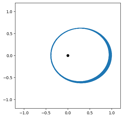
Now we apply RK4 to solve the system:

T, RV = RK4(va, np.array([1, 0, 0, 0.75]), 0, 0.1, 1000)

X_RK4 = RV[:,0]
Y_RK4 = RV[:,1]

plt.scatter([0],[0], color='k')
plt.plot(X_RK4, Y_RK4)
plt.xlim(-1.2,1.2)
plt.ylim(-1.2,1.2)
plt.gca().set_aspect('equal')

Leapfrog/Verlet Method

Leapfrog integrates the equations in a staggered manner:

(413)\[\begin{align} v_{n+1/2} &= v_n + \frac{1}{2} a(r_{n}) \Delta t, \\ r_{n+1} &= r_n + v_{n+1/2} \Delta t, \\ v_{n+1} &= v_{n+1/2} + \frac{1}{2} a(r_{n+1}) \Delta t. \end{align}\]

# Leapfrog/Verlet Method
def leapfrog(a, r0, v0, t0, dt, n):
    
    T = [t0]
    X = [r0[0]]
    Y = [r0[1]]
    U = [v0[0]]
    V = [v0[1]]

    ax, ay = a(X[-1], Y[-1])

    for _ in range(n):
        uh = U[-1] + ax * dt / 2
        vh = V[-1] + ay * dt / 2

        X.append(X[-1] + uh * dt)
        Y.append(Y[-1] + vh * dt)

        ax, ay = a(X[-1], Y[-1])

        U.append(uh + ax * dt / 2)
        V.append(vh + ay * dt / 2)

        T.append(T[-1] + dt)

    return np.array(T), np.array([X, Y]).T, np.array([U, V]).T

With leapfrog(), the “force” term is easier to implement:

def a(x, y):
    rr = x*x + y*y
    f  = -1 / (rr * np.sqrt(rr))
    return x * f, y * f

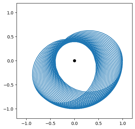
Running the leapfrog integration:

T, R, V = leapfrog(a, (1, 0), (0, 0.75), 0, 0.1, 1000)

X_lf = R[:,0]
Y_lf = R[:,1]

plt.scatter([0],[0], color='k')
plt.plot(X_lf,  Y_lf)
plt.xlim(-1.2,1.2)
plt.ylim(-1.2,1.2)
plt.gca().set_aspect('equal')

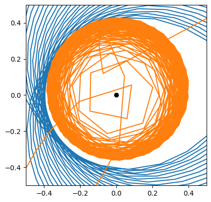
Comparing RK4 and Leapfrog

Now integrate this up to 2,000 dynamic time and compare between RK4 and leapfrog.

T, RV = RK4(va, np.array([1, 0, 0, 0.75]), 0, 0.1, 20_000)
X_RK4 = RV[:,0]
Y_RK4 = RV[:,1]

T, R, V = leapfrog(a, (1, 0), (0, 0.75), 0, 0.1, 20_000)
X_lf = R[:,0]
Y_lf = R[:,1]

plt.scatter([0],[0], color='k')
plt.plot(X_lf[10_000:11_000],  Y_lf[10_000:11_000])
plt.plot(X_RK4[10_000:11_000], Y_RK4[10_000:11_000])
plt.xlim(-0.5,0.5)
plt.ylim(-0.5,0.5)
plt.gca().set_aspect('equal')

Energy Computation and Conservation Analysis

To analyze the stability of our integrators, we compute the total energy:

(414)\[\begin{align} E = \frac{1}{2} (u^2 + v^2) - \frac{1}{\sqrt{x^2 + y^2}} \end{align}\]

def energy(R, V):
    X, Y = R[:,0], R[:,1]
    U, V = V[:,0], V[:,1]
    T = 0.5 * (U**2 + V**2)
    V = -1 / np.sqrt(X**2 + Y**2)
    return T + V

E_rk4 = energy(RV[:,:2], RV[:,2:])
E_lf  = energy(R, V)

plt.plot(T, E_rk4, label='RK4 Energy', linestyle='--')
plt.plot(T, E_lf,  label='Leapfrog Energy')
plt.xlabel('Time')
plt.ylabel('Total Energy')
plt.ylim(-10,10)
plt.legend()

<matplotlib.legend.Legend at 0x7f7acc13f1d0>

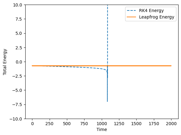
Conclusion

• RK4 provides high accuracy but does not conserve energy perfectly.

• Leapfrog maintains energy conservation better, making it suitable for long-term orbital simulations.